Parallelisation Using the parallel Package#
The following section is based off of Parallel Processing in R (University of Michigan) written by Josh Errickson at the University of Michigan. Additional information can be found in the R Parallel Package: PDF Documentation for the parallel package.
Overview#
Suppose you have found yourself in one of the following situations:
You have a function $f$ that you need to run many times for different input values.
You have a large set of functions $f_1, , \dots, , f_n$, $n>>1$, that you need to run, each for potentially many different input values.
If you’re like me, you’d probably prefer to get straight to analyzing the data produced by the functions as opposed to waiting around all day for them to finish running. This is where parallelization can help you.
We consider the case here where each function evaluation is completely independent of the others. In case 1 above, this is trivial because you’re just running the same function for many different input combinations. In the second scenario, this means that the functions are completely unrelated e.g. the output of one function is never used as the input to another.
A core on your computer can be thought of as an individual unit that can execute tasks. The vast majority of modern computers have multiple cores and parallelising your code involves sending independent jobs to different cores on your computer. In R one way of doing this is by using a concept called forking.
Forking (Will not work on Windows)#
Forking in R can be achieved using the parallel package, but first you should check that forking is actually supported within the environment in which you are developing your R code. Do do this, you can use the supportsMulticore() function from the parallelly package.
supportsMulticore()
[1] TRUE
In RStudio, depending on the version, the above may return FALSE, meaning forking is NOT supported, so you may not see any performance enhancements by using forking when running scripts in RStudio. Note I said may; as we will see below, using functions from the parallel package in Rstudio appear to behave well. However it is highly discouraged as the behaviour can be unexpected.
The advised way to use forking is to run R scripts using your terminal. Suppose you have a script called my-script.R. There are two ways to use your terminal to run my-script.R:
Initiate an R session directly in the terminal, in the same directory as
my-script.R, by typingR. Within the session typesource("my-script.R")Execute
my-script.Rdirectly using theRscriptcommand in your terminal, i.e. by typingRscript my-script.R
Exercise#
Implement the above procedure both inside and outside of RStudio, what are the results on your OS?
Forking - mclapply()#
First, let’s detect the number of cores available on our machine using detectCores() from the parallel package:
num_cores <- detectCores()
num_cores
[1] 12
On my machine, this returns 12, though on yours it may return something different. The output of detectCores() provides a useful guide on deciding how many cores to parallelise across, which can be specified in the mclapply() via the mc.cores argument. There are several important points here:
A value of two or greater for
mc.coresis necessary for parallelisation. Settingmc.cores = 1will disable parallelisation.It is not the case that choosing $n$ cores will result in a speed up of a factor of $n$.
Setting
mc.coreshigher than the number of available cores can actually slow down your code due to the overhead it creates. UsingdetectCores()/2is a useful starting point, and you can experiment from there.
Now let’s see mclapply() in action. Consider the following toy function, similar to the, which is used simply to represent an expensive function
slow_function <- function(n) {
  Sys.sleep(1)
  return(mean(rnorm(1000)))
}
Run using the regular lapply():
is <- 1:24
t1 <- system.time(lapply(is, slow_function))["elapsed"]
Run using parallelisation with mclapply() with four cores:
t4 <- system.time(mclapply(is, slow_function, mc.cores = 4))["elapsed"]
Run using parallelisation with mclapply() with eight cores:
t8 <- system.time(mclapply(is, slow_function, mc.cores = 8))["elapsed"]
Run using parallelisation with mclapply() with twelve cores:
t12 <- system.time(mclapply(is, slow_function, mc.cores = 12))["elapsed"]
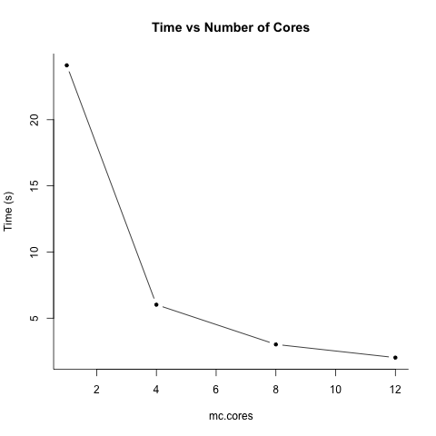
Plot the results
ts <- c(t1, t4, t8, t12)
cs <- c(1, 4, 8, 12)
plot(cs, ts, type = 'b', bty='l', xlab = "mc.cores", ylab = "Time (s)", pch = 20, main = "Time vs Number of Cores")
Example#
Try to use mclapply() on one of your own functions, both inside and outside of Rstudio. Do you notice any difference in speed? Note mclapply() only parallelises over one argument. For multivariate parallelisation, see mcmapply().