Model selection

Learning objectives

• Select different machine learning models in scikit-learn, and train them

• Understand that models have different characteristics, including flexibility, parameterisation, and more, which affects model selection and efficacy

• Explain the model flexibility/over-fit trade off

• Explain what model train and test error are, and how these relate to overfitting

Logistic regression

• Here is a simple binary classification task with a linear model.

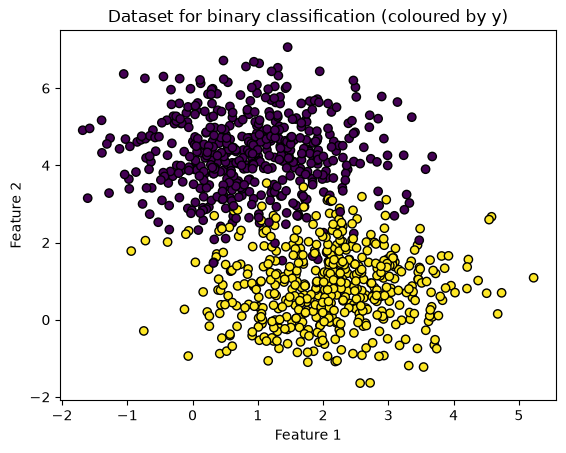
• First, we will create some binary classified data.

• Then we will train a model that can classify new points into one of the two classes.

import numpy as np
import matplotlib.pyplot as plt

from sklearn.datasets import make_blobs

# Generate binary classification dataset
X, y = make_blobs(n_samples=1000, centers=2, n_features=2, random_state=0)

print(f"X shape: {X.shape}, y shape: {y.shape}")

X shape: (1000, 2), y shape: (1000,)

print(f"X feature vector: {X[0]}")

X feature vector: [0.4666179  3.86571303]

print(f"y label: {y[0]}")

y label: 0

plt.scatter(X[:, 0], X[:, 1], c=y, edgecolors='k')
plt.xlabel('Feature 1')
plt.ylabel('Feature 2')
plt.title('Dataset for binary classification (coloured by y)')
plt.show()

So its time to train a model?

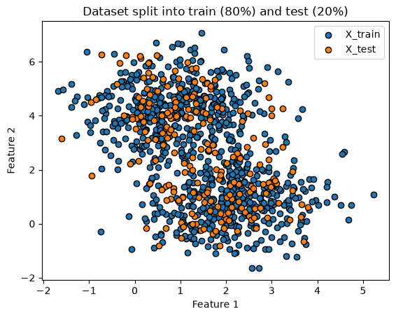
• Not quite. Lets split our X and y into X_train and X_test and y_train and y_test.

from sklearn.model_selection import train_test_split

X_train, X_test, y_train, y_test = train_test_split(X, y, test_size=0.2, random_state=42)

plt.scatter(X_train[:, 0], X_train[:, 1], label="X_train")
plt.scatter(X_test[:, 0], X_test[:, 1], label="X_test")
plt.xlabel('Feature 1')
plt.ylabel('Feature 2')
plt.title('Dataset split into train (80%) and test (20%)')
plt.legend()
plt.show()

• We will now train our model with X_train and y_train.

from sklearn.linear_model import LogisticRegression

model = LogisticRegression()
model.fit(X_train, y_train)

LogisticRegression()

In a Jupyter environment, please rerun this cell to show the HTML representation or trust the notebook.
On GitHub, the HTML representation is unable to render, please try loading this page with nbviewer.org.

• Now that we have a trained model, we can evaluate how the model performs on the test set that we held out at the start.

• Use the model to create predictions for the test data:

y_pred = model.predict(X_test)

• Then assess the accuracy against the true labels

from sklearn.metrics import accuracy_score

accuracy = accuracy_score(y_test, y_pred)
print(f'Accuracy: {accuracy:.2f}')

Accuracy: 0.95

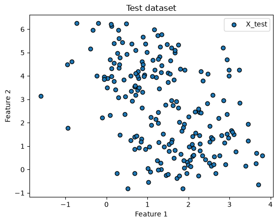
• Lets create some plots to show what is happening

plt.scatter(X_test[:, 0], X_test[:, 1], label="X_test")
plt.xlabel('Feature 1')
plt.ylabel('Feature 2')
plt.title('Test dataset')
plt.legend()
plt.show()

plt.scatter(X_test[:, 0], X_test[:, 1], c=y_pred, edgecolors='k')
plt.xlabel('Feature 1')
plt.ylabel('Feature 2')
plt.title('Test dataset coloured by model prediction')
plt.legend()
plt.show()

/tmp/ipykernel_2842/2276081007.py:5: UserWarning: No artists with labels found to put in legend.  Note that artists whose label start with an underscore are ignored when legend() is called with no argument.
  plt.legend()

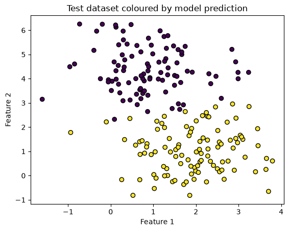
• Which points were incorrectly classified? We know that ~5% of 1000 were.

misclassified = X_test[y_test != y_pred]

plt.scatter(X_test[:, 0], X_test[:, 1], c=y_pred, edgecolors='k')
plt.scatter(misclassified[:, 0], misclassified[:, 1], color='red', marker='x', label='Misclassified')
plt.xlabel('Feature 1')
plt.ylabel('Feature 2')
plt.title('Test dataset coloured by model prediction')
plt.legend()
plt.show()

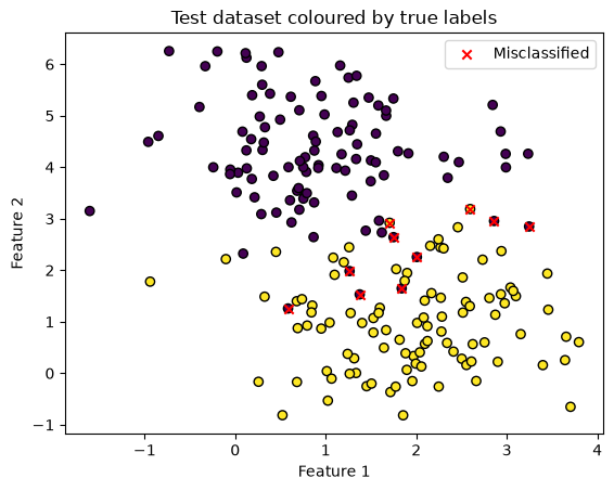
plt.scatter(X_test[:, 0], X_test[:, 1], c=y_test, edgecolors='k')
plt.scatter(misclassified[:, 0], misclassified[:, 1], color='red', marker='x', label='Misclassified')
plt.xlabel('Feature 1')
plt.ylabel('Feature 2')
plt.title('Test dataset coloured by true labels')
plt.legend()
plt.show()

Summary

• We have used a linear model to classify points into two classes.

• We achieves a 95% accuracy score on the test set: this means that given a new (representative) point, we should have a 95% chance of this point being accurately classified.

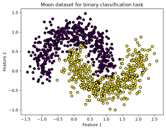
What happens when our data is not representative?

• If our input data distribution changes, our model performance will suffer.

• We can change our toy dataset fairly easily with scikit-learn.

• This is still a binary classification task. We can assess the classification performance of the model on the new dataset.

from sklearn.datasets import make_moons

X, y = make_moons(n_samples=1000, noise=0.2, random_state=42)
X_train, X_test, y_train, y_test = train_test_split(X, y, test_size=0.2, random_state=42)

y_pred = model.predict(X_test)
accuracy = accuracy_score(y_test, y_pred)

print(f'Accuracy: {accuracy:.2f}')

Accuracy: 0.50

• Our model is now as good (or bad) as flipping a coin.

• This makes sense: our data distribution has changed, and we need to re-train our model. Generalising to a random unseen dataset was never going to work!

• Lets create a linear model, train it on our new dataset, and assess its accuracy on the holdout test set.

model = LogisticRegression()
model.fit(X_train, y_train)

LogisticRegression()

In a Jupyter environment, please rerun this cell to show the HTML representation or trust the notebook.
On GitHub, the HTML representation is unable to render, please try loading this page with nbviewer.org.

y_pred = model.predict(X_test)
accuracy = accuracy_score(y_test, y_pred)

print(f'Accuracy: {accuracy:.2f}')

Accuracy: 0.86

Much better!

plt.scatter(X[:, 0], X[:, 1], c=y, edgecolors='k')
plt.xlabel('Feature 1')
plt.ylabel('Feature 2')
plt.title('Moon dataset for binary classification task')
plt.show()

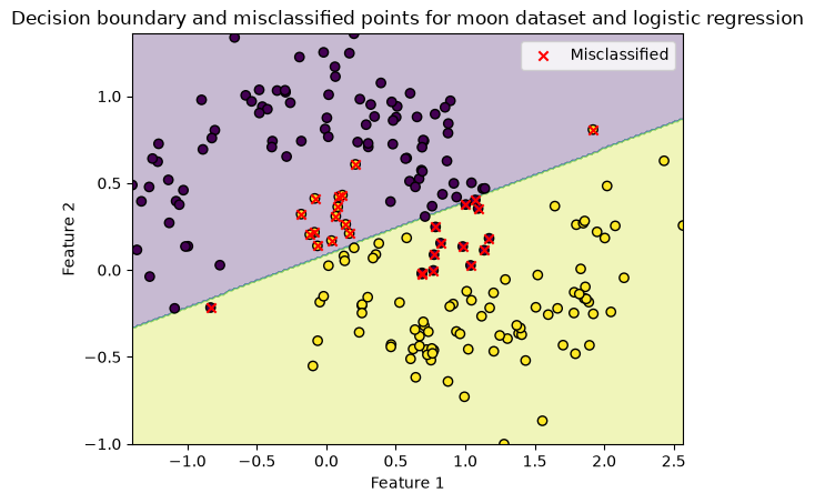
• Lets plot the misclassified points, but also the decision boundary

• For binary logistic regression, this is the line where the probability of belonging to a class is 0.5

def plot_boundary(X, y, model, misclassified, title):
    xx, yy = np.meshgrid(
        np.linspace(X[:, 0].min(), X[:, 0].max(), 200),
        np.linspace(X[:, 1].min(), X[:, 1].max(), 200),
    )
    Z = model.predict(np.c_[xx.ravel(), yy.ravel()]).reshape(xx.shape)
    plt.contourf(xx, yy, Z, alpha=0.3)
    plt.scatter(X[:, 0], X[:, 1], c=y, edgecolors="k")
    plt.scatter(
        misclassified[:, 0],
        misclassified[:, 1],
        color="red",
        marker="x",
        label="Misclassified",
    )
    plt.title(title)
    plt.xlabel("Feature 1")
    plt.ylabel("Feature 2")
    plt.legend()
    plt.show()

# Find the misclassified points as before
misclassified = X_test[y_test != y_pred]

title="Decision boundary and misclassified points for moon dataset and logistic regression"
plot_boundary(X_test, y_test, model, misclassified, title)

Changing model

• We can potentially get improved performance if we select a new model

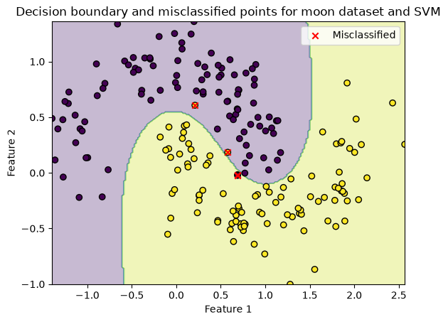
• Lets use an SVM (support Vector Machine) with a radial basel function kernel.

• This can model non-linear decision boundaries.

from sklearn.svm import SVC

# Train SVM with RBF kernel
model = SVC(kernel='rbf', gamma='scale')
model.fit(X_train, y_train)

SVC()

In a Jupyter environment, please rerun this cell to show the HTML representation or trust the notebook.
On GitHub, the HTML representation is unable to render, please try loading this page with nbviewer.org.

# Predict and evaluate as before
y_pred = model.predict(X_test)
accuracy = accuracy_score(y_test, y_pred)

print(f'Accuracy: {accuracy:.2f}')

Accuracy: 0.98

• Great! We improved our prediction accuracy by 11%.

• Lets visualise the classification on the test set again, to show the non-linear decision boundary

# Identify misclassified points as before
misclassified = X_test[y_test != y_pred]

title="Decision boundary and misclassified points for moon dataset and SVM"
plot_boundary(X_test, y_test, model, misclassified, title)