Style Guides and Linters

/Users/cc1333/Library/Python/3.9/lib/python/site-packages/rpy2/ipython/rmagic.py:77: UserWarning: The Python package `pandas` is strongly recommended when using `rpy2.ipython`. Unfortunately it could not be loaded (error: No module named 'pandas'), but at least we found `numpy`.
  warnings.warn('The Python package `pandas` is strongly '

%%R
suppressPackageStartupMessages({
  suppressMessages({
    library(dplyr)
    library(styler)
  })
})

Style Guides and Linters#

The Tidyverse Style Guide#

A style guide is a set of rules that embed consistency into your code. One such set of rules are contained in the Tidyverse Style Guide. These rules are essentially just opinions, since there are no hard-and-fast rules to the way you write your code, and there are many different style guides available. We have chosen to discuss the Tidyverse style guide because of its popularity. We could not feasibly cover every point in the Tidyverse Style Guide within this session, but we hope to emphasise some of the main points and tie them together with an example so you can bring the ideas back to your own code after the session. Complete details can be found in the style guide.

Being conscious of consistency in your code can go a long way in improving the ease of collaboration and the impact of your code on your research. We will approach consistency from three levels of increasing granularity:

File name
Structure implemented within a file
Syntax used within file

File Naming and Structure#

The first simple yet important aspect of an R file is its name. When naming your file you should:

Give your file a descriptive name
Give your file the extension .R (not .r)
Avoid whitespace.

Suppose we have a script that fits a linear model; calling this file some file.r violates all of the above. Naming the file fit-linear-model.R will make it much easier to locate.

If you have a sequence of files that are intended to be run in a specific order, number them to indicate this. For example, 01-exploratory-analysis.R, 02-fit-models.R, 03-plot-results.R.

If you have to import a set of libraries, do so at the beginning of the file using library() as opposed to loading them sporadically throughout the file.

Often, using comments such as # ---------- ... ------------ can be useful to increase readability and indicate the purpose of each sub-section in the script. For example, one way of organising a small script could be as follows:

%%R
# ---------- loading libraries ---------

# ---------- defining functions --------

# ---------- performing analysis -------

# ---------- saving and plotting results ------------

NULL

Note, in R using the project structure or even creating your own R package can be useful for more involved analyses, though we do not cover those topics here.

File Syntax#

Variables and Functions#

Naming conventions extend from the file itself to the variables, functions and classes in your code; these should be consistent.

Variable and function names should only contain lowercase letters, numbers and underscores. In particular, names should not contain white space. If a variable name contains multiple words, separate them using underscores. For example:

%%R
# good
string_one <-  "hello world!"

# bad
StringOne <-  "hello world!"

# bad
stringone <-  "hello world!"

Also, never use the names of built in functions or variables e.g. T, mean, pi, sum etc.

Assignment#

Use <- for assignment instead of =.

%%R
# good
greeting <- "hello" 

# bad
greeting = "hello"

Semi-colons#

Don’t use them

%%R
# bad
x <-  1; y <- 2; z <- 3;

# good
x <- 1
y <- 2
z <- 3

Horizontal Spacing#

Commas: space as you would in normal English i.e. a space after, and only after, the comma.

%%R
# bad
ones_matrix <- matrix( 1, 10 ,10 )
ones_matrix[ , 1]

# good
twos_matrix <- matrix(2, 10, 10)
twos_matrix[, 1]

 [1] 2 2 2 2 2 2 2 2 2 2

Parentheses: avoid spaces before and after parentheses in function calls, but do include them before and after conditional statements.

%%R
word_print_bad <- function (word) {
  if(word){
    print( word ) 
  }
}

word_print_good <- function(word) {
  if (word) {
    print(word) 
  }
}

Vertical Spacing#

Excessive whitespace should be avoided, but no whitespace at all is equally as bad. The style guide suggests the following:

Avoid empty lines at the start or end of functions.
Only use a single empty line when needed to separate functions or pipes.
It often makes sense to put an empty line before a comment block, to help visually connect the explanation with the code that it applies to.

Functions#

Setting up a function quickly#

Functions are an integral part of R; the skeleton code for a function in R is:

%%R
name <- function(variables) {
  
}

In RStudio, you can set this up quickly by typing fun and hitting the tab key twice on your keyboard.

Returning#

You only need to write return in a function for an early return. R returns the last evaluated expression by default.

%%R
# good
celcius_to_fahrenheit_good <- function(temperature){
  temperature*(9/5) + 32  
}

# bad
celcius_to_fahrenheit_bad <- function(temperature){
  return(temperature*(9/5) + 32)
}

celcius_to_fahrenheit_good(-20)
celcius_to_fahrenheit_bad(-20)

[1] -4

Example of early return:

%%R
random_function <- function(){
  x <- runif(1)
  if (x < 0.25){
    message("** The number was less than 0.25")
    return(x)
  } else {
    message("** The number was greater than 0.25")
    random_function()
  }
}

xx <- random_function()
xx

[1] 0.1492978

** The number was greater than 0.25
** The number was less than 0.25

Function Arguments#

In R, a function’s arguments are typically either:

Data being computed on (we can omit the names here)
Computation details (we typically use the full names of these)

%%R
# Good
mean(1:10, na.rm = TRUE)

# Bad
mean(x = 1:10, , FALSE)
mean(, TRUE, x = c(1:10, NA))

[1] 5.5

Use the full names of the arguments you specify. In R you can use partial matching by specifying a unique prefix of a function argument, but this should be avoided as it can create unnecessary ambiguity.

%%R
# bad
mean(c(1:10, NA), n = TRUE)
mean(c(1:10, NA), na = TRUE)
mean(c(1:10, NA), na. = TRUE)
mean(c(1:10, NA), na.r = TRUE)

# good
mean(c(1:10, NA), na.rm = TRUE)

[1] 5.5

Exercise#

Consider the following two versions of R code that perform the same task. Discuss in groups what is good about each implementation and what could be improved.

%%R
# file name: my code.r

# this script does stuff
library(ggplot2);library(dplyr)

dat = mtcars; DATA2=dat %>% select(mpg);result=mean(DATA2$mpg)
PrintMean <- function(d){
  m <- mean(d$mpg); print(paste("The mean is:",m)); return(m)
}

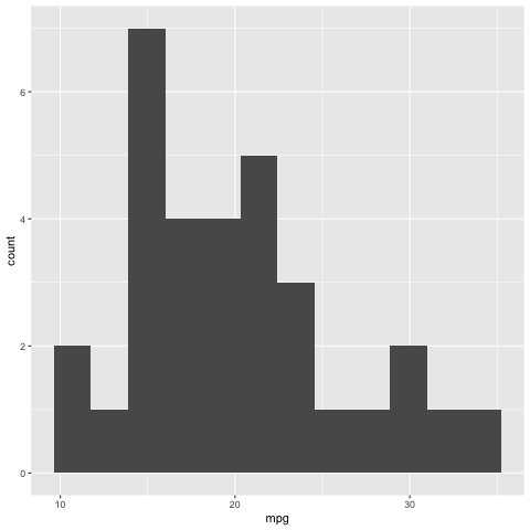
ShowHist <- function(d,bars=10){
  ggplot(data = d,aes(x= mpg))+geom_histogram(bins=bars)
}

x = PrintMean(d=dat)
ShowHist(dat, ba=12)

[1] "The mean is: 20.090625"

../../_images/cf006501714b329430727919ee91ed51a8e52719c4000052fd0149ddf935e03a.png

%%R
# file name: calculate_mpg_summary.R

# ----------------------------------------
# Load required libraries
# ----------------------------------------
library(ggplot2)
library(dplyr)

# ----------------------------------------
# Prepare data
# ----------------------------------------
mtcars_data <- mtcars
mpg_data <- mtcars_data %>% select(mpg)

# ----------------------------------------
# Function to calculate mean MPG
# ----------------------------------------
print_mean_mpg <- function(data) {
  mean_value <- mean(data$mpg)
  print(paste("The mean MPG is:", mean_value))
  mean_value
}

# ----------------------------------------
# Function to show histogram of MPG
# ----------------------------------------
show_histogram <- function(data, bins = 10) {
  ggplot(data = data, aes(x = mpg)) +
    geom_histogram(bins = bins)
}

# ----------------------------------------
# Run analysis
# ----------------------------------------
mean_mpg <- print_mean_mpg(mtcars_data)
show_histogram(data = mtcars_data, bins = 12)

[1] "The mean MPG is: 20.090625"

The Styler and lintr packages#

The styler and lintr package are two useful packages for formatting your code according to the Tidyverse style guide. You can install them from CRAN in the usual way:

install.packages("styler")
install.packages("lintr")

Exercise#

Paste the file my code.r from the example above into a new R file. Peruse the documentation of the styler package and experiment with the style_file function. How does it work on the my code.rexample?

Do the same with the lintr package, using the lint function. How does it work with the my code.rexample?

Style Guides and Linters

Contents

Style Guides and Linters#

The Tidyverse Style Guide#

File Naming and Structure#

File Syntax#

Variables and Functions#

Assignment#

Semi-colons#

Horizontal Spacing#

Vertical Spacing#

Functions#

Setting up a function quickly#

Returning#

Function Arguments#

Exercise#

The Styler and lintr packages#

Exercise#