Unsupervised learning

Learning objectives

• Recap what unsupervised learning is

• Explain how this relates to supervised learning, especially the main differences

• Perform K-means clustering, a simple unsupervised learning algorithm, on sample data

Recap

• In unsupervised learning, models learn from unlabelled data (i.e. without explicit supervision).

• The goal is to learn (often hidden) patterns or structures in the data.

• We use unsupervised learning for clustering, dimensionality reduction, anomaly detection, and more.

K-means clustering

• This type of algorithm tries to assign class labels (i.e. generate clusters) from unlabelled data.

• While there are many types of algorithms that generate clusters, K-means is a great place to start due to its simplicity (much like how we defaulted to linear regressions in previous notebooks).

How does it work?

The algorithm is quite simple. To generate k clusters from a dataset, it minimises the variance within each cluster.

1. Create k cluster centroids randomly

2. Assign each data point to the nearest centroid

3. Compute new centroids as the mean of the assigned points

4. Repeat steps 2 and 3 until the centroids stabilise (i.e. they do not move significantly)

omput

import numpy as np
import matplotlib.pyplot as plt
from sklearn.cluster import KMeans
from sklearn.datasets import make_blobs

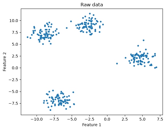
# Generate some data
X, y = make_blobs(n_samples=300, centers=4, cluster_std=1.0, random_state=42)

plt.scatter(X[:, 0], X[:, 1], s=10)
plt.title("Raw data")
plt.xlabel('Feature 1')
plt.ylabel('Feature 2')
plt.show()

def kmeans_and_plot(X, n_clusters, title):
    # Apply k-means
    kmeans = KMeans(n_clusters, random_state=42)
    kmeans.fit(X)
    y_kmeans = kmeans.predict(X)

    # Plot data coloured by k-means
    plt.scatter(X[:, 0], X[:, 1], c=y_kmeans, s=10, cmap="viridis")
    plt.scatter(
        kmeans.cluster_centers_[:, 0],
        kmeans.cluster_centers_[:, 1],
        c="red",
        marker="X",
        s=100,
        label="Centroids",
    )
    plt.title(title)
    plt.xlabel('Feature 1')
    plt.ylabel('Feature 2')
    plt.legend()
    plt.show()

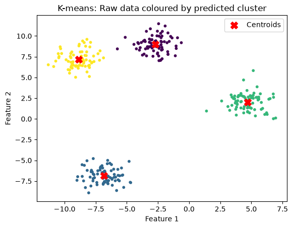
n_clusters = 4
title="K-means: Raw data coloured by predicted cluster"
kmeans_and_plot(X, n_clusters, title)

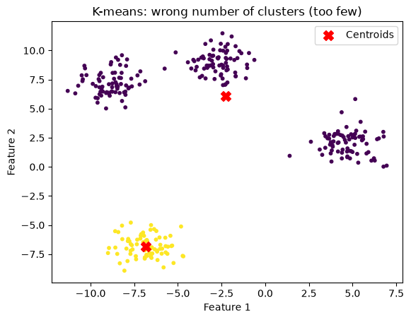
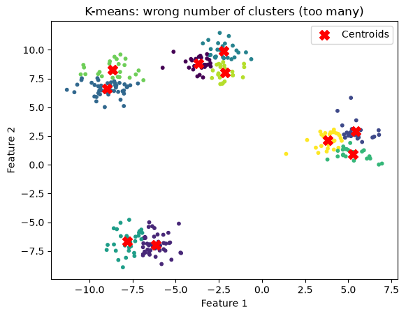
What happens if we have the wrong k?

• Here we could easily see 4 clusters, and specify k = 4.

• But what if we provide the wrong k?

n_clusters = 2
title="K-means: wrong number of clusters (too few)"
kmeans_and_plot(X, n_clusters, title)

n_clusters = 10
title="K-means: wrong number of clusters (too many)"
kmeans_and_plot(X, n_clusters, title)

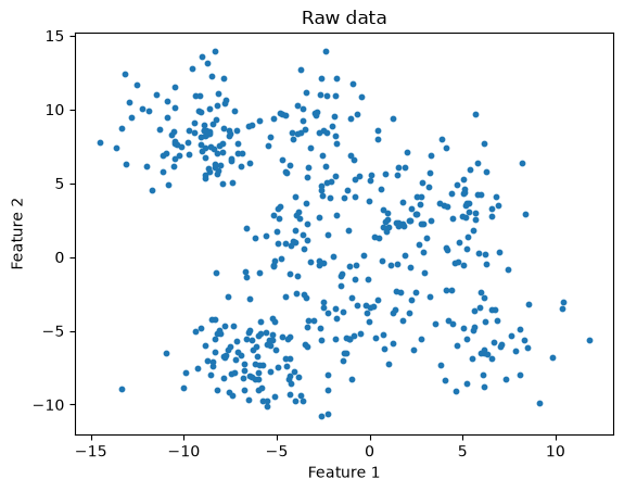
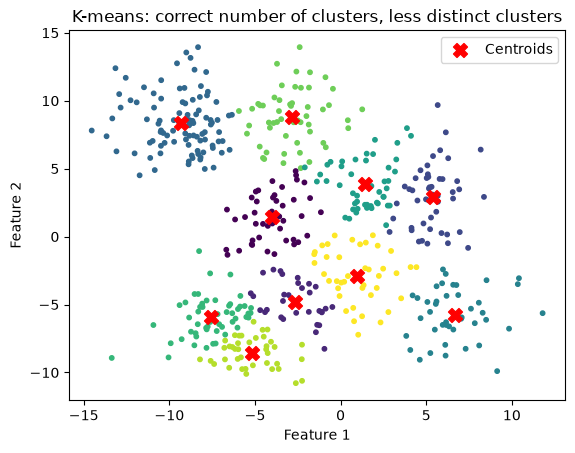
• Finally, what happens if we have a less distinct data set?

# Generate some data
X, y = make_blobs(n_samples=500, centers=10, cluster_std=2.0, random_state=42)

plt.scatter(X[:, 0], X[:, 1], s=10)
plt.title("Raw data")
plt.xlabel('Feature 1')
plt.ylabel('Feature 2')
plt.show()

n_clusters = 10
title="K-means: correct number of clusters, less distinct clusters"
kmeans_and_plot(X, n_clusters, title)

Determining the number of clusters

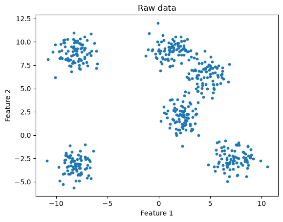
• We can attempt to calculate the number of clusters using the elbow method.

• This is not perfect, as shown below

# Generate some data
X, y = make_blobs(n_samples=500, centers=6, cluster_std=1., random_state=32)

plt.scatter(X[:, 0], X[:, 1], s=10)
plt.title("Raw data")
plt.xlabel('Feature 1')
plt.ylabel('Feature 2')
plt.show()

def elbow_method_and_plot(X, k_range, title, random_state=42):

    # Store within cluster sum of squares (inertia)
    wcss = []
    for k in k_range:
        kmeans = KMeans(n_clusters=k, random_state=random_state)
        kmeans.fit(X)

        # Store inertia
        wcss.append(kmeans.inertia_)

    # Plot the elbow curve
    plt.figure(figsize=(8, 5))
    plt.plot(k_range, wcss, marker='o', linestyle='-')
    plt.xlabel("Number of clusters k")
    plt.ylabel("Within cluster sum of squares (WCSS)")
    plt.title(title)
    plt.xticks(k_range)
    plt.show()

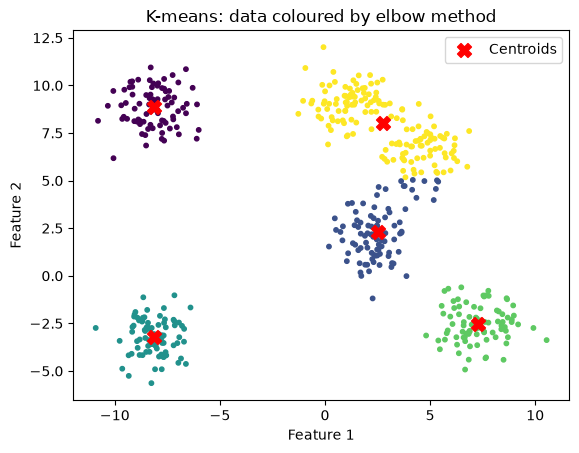
k_range = range(1, 11)
title = "Elbow method for finding k"
elbow_method_and_plot(X, k_range, title, random_state=42)

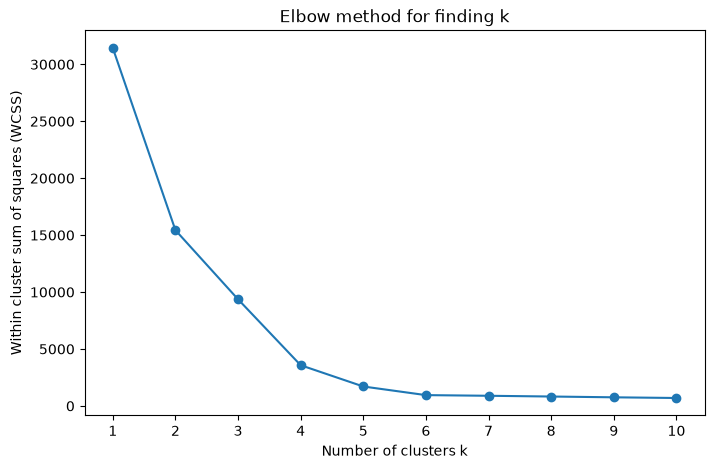
n_clusters = 5
title="K-means: data coloured by elbow method"
kmeans_and_plot(X, n_clusters, title)

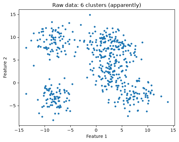
• When the clusters are less distinct, the elbow method might be less helpful:

# Generate some data
X, y = make_blobs(n_samples=500, centers=6, cluster_std=2, random_state=32)

plt.scatter(X[:, 0], X[:, 1], s=10)
plt.title("Raw data: 6 clusters (apparently)")
plt.xlabel('Feature 1')
plt.ylabel('Feature 2')
plt.show()

k_range = range(1, 11)
title = "Elbow method for finding k"
elbow_method_and_plot(X, k_range, title, random_state=42)

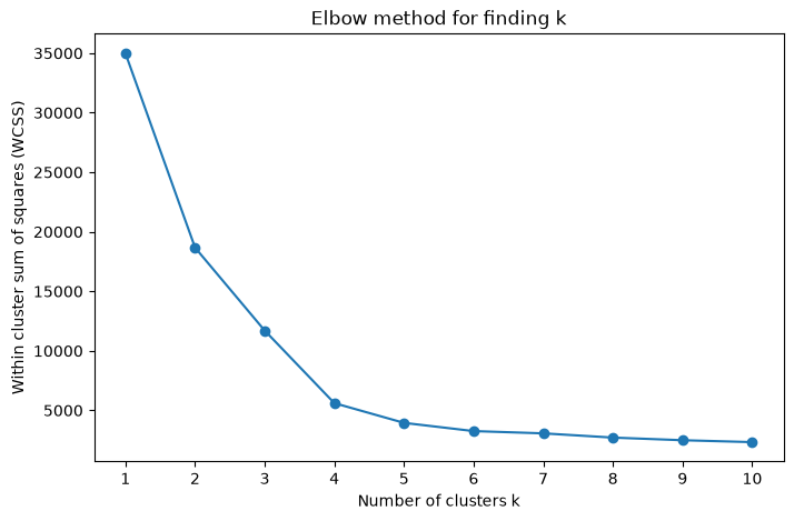
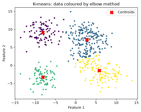
n_clusters = 4
title = "K-means: data coloured by elbow method"
kmeans_and_plot(X, n_clusters, title)

K-means Animation

Below is a animation of K-means, showing each iteration of the algorithm. Notice how the centroids get closer and closer to what a human might label as a ‘blob centre’ with each step. You should also notice how the centroids move in each iteration, they move to the centre of the points assigned to them.