Writing Functions in R#
Author: Ruxandra Neatu (GitHub: NeatuR) and Thomas Hawes (GitHub: thawes-rse)
License: Creative Commons Attribution-ShareAlike 4.0 International license (CC BY-SA 4.0).
Course Objectives#
Understand and write functions in R.
Understand the difference between local and global variables.
Apply best practices to avoid common programming errors related to variable usage.
Motivation and Background#
A function is a reusable block of code that takes inputs (described by parameters), performs operations and returns an output.
Using functions in your code has several advantages:
Reduce redundancy: by writing a function once and reusing it whenever needed, you avoid repeating the same code in muliple places.
Enhances modularity: functions allow you to structure your code into modules, each performing a specific task, making development and maintenance easier.
Facilitates testing: because functions are self-contained, they can be tested individually to ensure they work correctly before integrating them into the larger program.
Improves readability: well-named functions break down complex scripts into clear, logical components, making your code easier for you and others to read and understand.
This short course is a practical introduction to writing functions in R. It covers key concepts to help you structure code, avoid repetition, and write clearer scripts. For more in-depth learning, including default parameter values and other topics, see the Software Carpentry “Creating Functions”.
Before Writing Functions#
When writing functions, give them meaningful names. The format
verb_nouncan be useful, such asadd_summaries.Always document the inputs and outputs with comments to explain what the function expects and returns. Also document any other ‘side effects’, e.g. messages printed to the console, files written or global variables modified (see later about global variables).
To keep your project organised, save functions in separate scripts within a dedicated directory (for example, an
R/folder).You can import these functions into your main script using
source("R/file_name.R"), which makes them available for use in your workflow.
Basic Syntax#
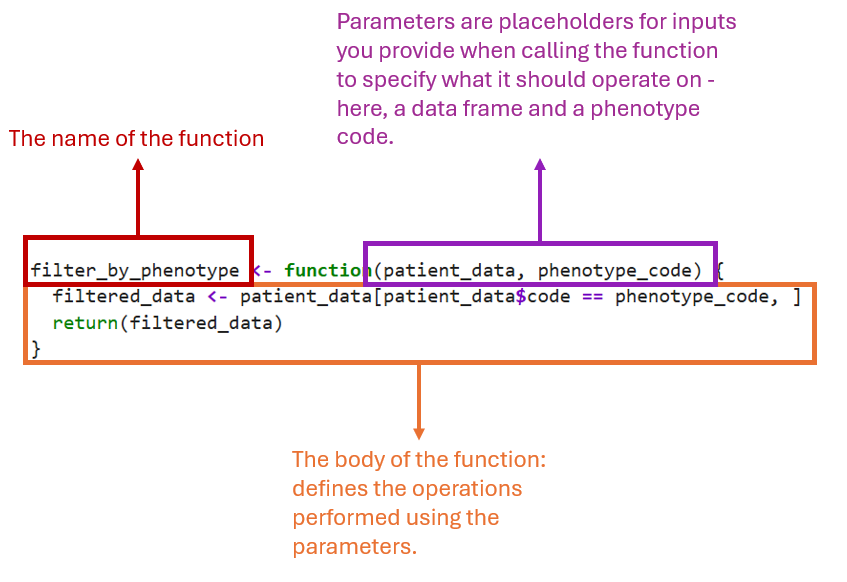
Let’s take an example of a function that aims to subset a table of patient data (patient_data) by the phenotype_code found in the column named code. We start by defining the function first:
filter_by_phenotype <- function(patient_data, phenotype_code) {
  filtered_data <- patient_data[patient_data$code == phenotype_code, ]
  return(filtered_data)
}
In the diagram below, the function is broken down into 3 components:
The name of the function:
filter_by_phenotype.The function parameters:
patient_data,phenotype_code.The body of the function:
  filtered_data <- patient_data[patient_data$code == phenotype_code, ]
  return(filtered_data)
In order to use the function on an actual dataframe of patient data (called data, say) and phenotype code (101, say), the function needs to be called as follows:
Write the name of the function (in this case
filter_by_phenotype).Replace the parameters
patient_dataandphenotype_codewith the actual variables/values (dataand phenotype code101)
filter_by_phenotype(data, 101)
As an example, let’s store the filtered table into an object called result and print it:
result <- filter_by_phenotype(data, 101)

print(result)
Where the components are:
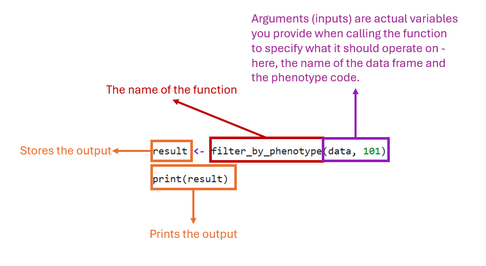
Note: The filtered table will be stored in the result and the initial table used as input data will be unchanged.
Exercise: Write your own function#
Write a function that takes in as an argument a dataframe
datawith column namexcontaining numbers. The function should return a dataframe with a new column, calledx_pow2, that is the square of the values in columnx. (E.g. ifxis a column with values1, 2, 3thenx_pow2should contain1, 4, 9. Make sure to give your function a good name!Evaluate your function from 1 on some different dataframes (which you create) to check that it works.
Now modify your function to take in two arguments: a dataframe
dataas before, but also an integern. The function should now return a dataframe with a new columnx_pow{n}which raises the values inxto thenth power. (For example, ifn=3the new column should be calledx_pow3.) Make sure the function has a good name! Try your function with different values fornto check it works.
Exercise: Guess the output#
Consider the following function, that takes a dataframe with a column called age and sets all the rows to have a particular age:
set_age <- function(data, new_age) {
    data$age <- new_age
}
Now consider the following dataframe:
df <- data.frame(name = c("Alice", "Bob", "Claire", "David"),
                 age = c(21, 23, 34, 43))
What do you think will be printed by the following code?
set_age(df, 99)
print(df)
Check your answer by running the code yourself.
Local vs Global Variables#
When writing functions in R, it is important to understand the difference between local and global variables.
Local Variable |
Global Variable |
|---|---|
Defined inside a function |
Defined outside of functions |
Accessible only within that function |
Accessible from anywhere |
Created each time the function runs |
Exists until removed from the environment |
For example, in the following function, result is a local variable because it is created inside the function and only exists there:
sum_numbers <- function(x) {
  result <- x + 5
  return(result)
}
Calling sum_numbers(10) will return 15:
sum_numbers(10)
On the other hand, in the code below z is an example of a global variable:
z <- 100

sum_numbers <- function(x) {
  result <- x + z
  return(result)
}
Here, z is a global variable because it is defined outside the function. It can still be used within the body of the function. For example, calling sum_numbers(5) will return 105:
sum_numbers(5)
However, if z changes (e.g. z <- 200), the output of the function will also change accordingly:
z <- 200
sum_numbers(5)
It is recommended that functions be self-sufficient and use local variables, as relying on global variables can lead to errors such as accidental overwriting of the global variables and/or unexpected changes in values, which makes it difficult to debug functions that depend on global variables. A better practice is to instead have an extra parameter for the global variable and then pass the variable into the function this way:
# Provide an extra paramter `y` to take the place of the global variable:
sum_numbers <- function(x, y) {
    result <- x + y
    return(result)
}

# Now call the function with the global variable z as an argument:
sum_numbers(5, z)
Functions in Practice: Life Sciences Data#
This section explores how functions are applied to analyse and interpret data in the life sciences. We use a dataset derived from a clinical dataset of gallstone diagnoses: you can download the data as a CSV file (which is made available under the Creative Commons Attribution 4.0 International licence). Using this dataset, you will learn how functions break down complex tasks into smaller, reusable steps.
About the data
The data we will use is derived from Esen, I., Arslan, H., Aktürk, S., Gülşen, M., Kültekin, N., & Özdemir, O. (2024). Gallstone [Dataset]. UCI Machine Learning Repository. https://doi.org/10.1097/md.0000000000037258. The original data is licensed under a Creative Commons Attribution 4.0 International licence and you can download it from the UC Irvine Machine Learning Repository. Our derived version of the data only includes a subset of the original columns, which have been renamed to make them easier to work with in code. We have also randomly removed some of the body mass index (BMI) values rows in the data, for the purposes of instruction.
If you wish to download the script and raw data used to create our derived dataset, you can download them as a zip archive.
Use of
dplyrThis part of the notes assumes you have the R package
dplyrinstalled.
The data was collected from the Internal Medicine Outpatient Clinic of Ankara VM Medical Park Hospital. Each row corresponds to an individual and includes an indicator of whether the individual had gallstones present (Gallstone_status = 1) or not (Gallstone_status = 0). There are several other variables (columns) in the dataset, including body mass index (BMI).
Suppose we want to do the following:
Categorise the samples (rows) into discrete BMI categories, according to the following cases:
Normal: 18.5 <= BMI < 25
Overweight: 25 <= BMI < 30
Obese: 30 <= BMI
Underweight: BMI < 18.5
Calculate averages (mean) of different columns in the dataset for each of the BMI categories (e.g. average incidence of diabetes in each of the BMI categories).
The code below calculates the averages for each BMI category of three different columns:
Total_body_fat_pct: total body fat percentageDiabetes: whether the subject has diabetes (1) or not (0)Total_cholesterol: total cholesterol in blood (mg/dL)
Later, we will see a way we can write functions to simplify the code.
data <- read.csv("data/r_functions/gallstone.csv")

# Filter the data to keep only rows where BMI is not missing
BMI_data <- data |>
  dplyr::filter(!is.na(BMI))

# Issue warning if any rows were dropped due to missing BMI
if (nrow(BMI_data) < nrow(data)) {
  n_dropped_rows = nrow(data) - nrow(BMI_data)
  warning("Dropped ", n_dropped_rows, " rows with missing BMI readings")
}

# Add BMI categories to the data
BMI_levels <- c("Normal", "Overweight", "Obese", "Underweight")
BMI_data <- BMI_data |>
  dplyr::mutate(
    BMI_cat = dplyr::case_when(
      BMI >= 18.5 & BMI < 25 ~ "Normal",
      BMI >= 25 & BMI < 30 ~ "Overweight",
      BMI >= 30 ~ "Obese",
      BMI < 18.5 ~ "Underweight"
    )
  ) |>
  dplyr::mutate(BMI_cat = factor(BMI_cat, levels = BMI_levels))

# Calculate average body fat percentage for each BMI category
body_fat_averages <- BMI_data |>
  dplyr::group_by(BMI_cat) |>
  dplyr::summarise(
    Total_body_fat_pct_mean = mean(Total_body_fat_pct, na.rm = TRUE)
  )

# Calculate average incidence of diabetes for each BMI category
diabetes_averages <- BMI_data |>
  dplyr::group_by(BMI_cat) |>
  dplyr::summarise(
    Diabetes_mean = mean(Diabetes, na.rm = TRUE)
  )

# Calculate average cholesterol for each BMI category
cholesterol_averages <- BMI_data |>
  dplyr::group_by(BMI_cat) |>
  dplyr::summarise(
    Total_cholesterol_mean = mean(Total_cholesterol, na.rm = TRUE)
  )
Warning message:
"Dropped 13 rows with missing BMI readings"
Exercise: breaking it down into functions#
Before you go any further, try to think about what function(s) you could create to simplify the above code. There’s no right or wrong answer here: the main thing is to just get you thinking before we present our own solution below. You might like to consider:
Where is there duplication in the code i.e. which parts look very similar to each other?
Can you see logical ‘dividing lines’ in the code i.e. places where it’s doing a qualitatively ‘new’ thing?
Decomposing into functions#
Below one possible way to use functions to rewrite the code above. We have created two functions:
add_BMI_categoriesadds the columnBMI_catof BMI categories to a dataframe with BMI scores.average_over_BMI_categoriescalculates the mean of a given column for each BMI category, for a dataframe with aBMI_catcolumn.
First let’s show the code for the functions:
#' Add a column of BMI categories
#'
#' The following ranges are used for the categorization:
#'
#' Normal:      18.5 <= BMI < 25
#' Overweight:  25 <= BMI < 30
#' Obese:       30 <= BMI
#' Underweight: BMI < 18.5
#'
#' If `data` has rows that are missing a BMI score then these rows will be
#' dropped and a warning message displayed.
#'
#' @param data A dataframe containing a column 'BMI' of numerical BMI scores.
#'
#' @returns A dataframe with a new factor column 'BMI_cat', with the levels
#'   ordered "Normal", "Overweight", "Obese", "Underweight".
add_BMI_categories <- function(data) {
  BMI_data <- data |>
    dplyr::filter(!is.na(BMI))

  if (nrow(BMI_data) < nrow(data)) {
    n_dropped_rows = nrow(data) - nrow(BMI_data)
    warning("Dropped ", n_dropped_rows, " rows with missing BMI readings")
  }

  BMI_levels <- c("Normal", "Overweight", "Obese", "Underweight")
  BMI_data <- BMI_data |>
    dplyr::mutate(
      BMI_cat = dplyr::case_when(
        BMI >= 18.5 & BMI < 25 ~ "Normal",
        BMI >= 25 & BMI < 30 ~ "Overweight",
        BMI >= 30 ~ "Obese",
        BMI < 18.5 ~ "Underweight"
      )
    ) |>
    dplyr::mutate(BMI_cat = factor(BMI_cat, levels = BMI_levels))

  return(BMI_data)
}

#' Average a column over BMI categories
#'
#' The average values of the column is calculated as the mean after removing rows
#' with missing values.
#'
#' @param data A dataframe containing a column 'BMI_cat' of discrete BMI
#'   categories.
#' @param column The column name (as a string) to calculated the BMI category
#'   averages for.
#'
#' @returns A dataframe of the BMI category mean values for the given `column`,
#'   with one row per BMI category. The name of averages column takes the form
#'   '{column}_mean' where {column} is the name provided through `column`.
average_over_BMI_categories <- function(data, column) {
  avg_column <- paste0(column, "_mean")
  summarised <- data |>
    dplyr::group_by(BMI_cat) |>
    dplyr::summarise(
      "{avg_column}" := mean(.data[[column]], na.rm = TRUE)
    )
  return(summarised)
}
Now let’s look at our original script, rewritten to use the functions:
data <- read.csv("data/r_functions/gallstone.csv")

# Add BMI categories (after dropping missing BMI values)
BMI_data <- add_BMI_categories(data)

# Calculate averages of different columns over BMI categories
body_fat_averages <- average_over_BMI_categories(BMI_data, "Total_body_fat_pct")
diabetes_averages <- average_over_BMI_categories(BMI_data, "Diabetes")
cholesterol_averages <- average_over_BMI_categories(BMI_data, "Total_cholesterol")
Warning message in add_BMI_categories(data):
"Dropped 13 rows with missing BMI readings"
Here are some remarks on the above use of functions:
We have used
average_over_BMI_categoriesto remove dupication in our original code: the process of grouping by BMI category and calculating an average.The function
add_BMI_categoriesis used to ‘encapsulate’ a logically consistent part of the code that is potentially useful on its own: namely, adding the BMI categories as a new column (after dropping missing BMI values)We have given our new functions descriptive names: when you read them being used in our modified version of the code, you can get a good sense of what the code is doing without needing to study how the functions are implemented. This is sometimes called writing code that is self-documenting.
Exercise: Adding new summary statistics#
Suppose we now want to also calculate the minimum and maximum values of the Total_body_fat_pct, Diabetes and Total_cholesterol columns within each of the BMI categories, in addition to the mean. How would you do this is the original code? How would you do this using the functions above? How has breaking down the code into functions helped in this case?
Exercise: Alternatives#
The functions we chose to write are just one way to rewrite the original code. Take the original code and come up with a new way to rewrite it by defining different function(s) to what we defined above. (You may reuse at most one of our functions if you wish.) For this exercise, don’t be afraid to define functions that you feel are ‘worse’ than ours: the main point is to practice looking at some code and coming up with ways to restructure it to use functions.
If you feel your new way of doing this is better or worse than ours, can you articulate why you think this is the case? (Don’t worry if you find this difficult! )