Acceleration via Rcpp (advanced)#
Overview#
C++ is a high-performance, general-purpose programming language that extends C with object-oriented, generic, and functional programming features. If you don’t know what those are, or have never used C++ before, do not worry. For us the most important point to note is that it can provide a fast alternative to R and can be integrated into our R code. In fact, under the hood, many of the base R functions are themselves written in C. In addition, many R packages on CRAN contain functions written in C++.
The easiest way to use C++ code in an R environment is through the Rcpp package. On MacOS and Linux systems, the Rcpp package is likely to be setup and loaded correctly after executing install.packages('Rcpp'), followed by library(Rcpp). On a windows OS, you may need to follow the instructions Rtools for Windows (CRAN) to download Xtools.
You can check Rcpp is set up correctly by trying the following:
evalCpp("2+2")
[1] 4
Example: Estimating Pi#
Suppose we want to estimate the value of pi. One way of doing this is to use Monte Carlo sampling.
Consider a quarter-circle of radius 1 inside the unit square \( [0,1] \times [0,1].\) The equation for the quarter-circle is
Since the area of the full circle is \( \pi \), the quarter-circle has an area of \( \pi/4 \). By randomly sampling points inside the square and checking how many fall inside the quarter-circle, we can estimate \( \pi \) using:
where \( M \) is the number of points inside the quarter-circle, and \( N \) is the total number of points sampled.
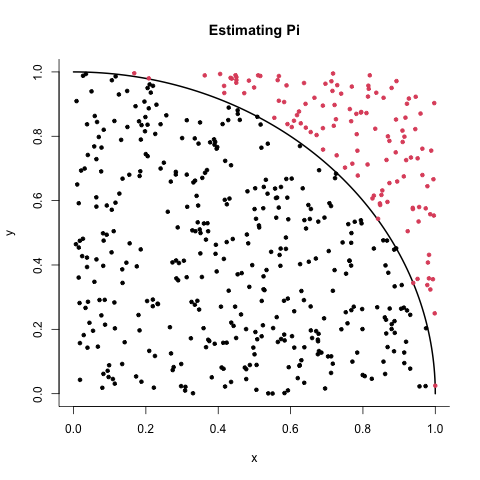
We can plot this set-up:
# Define the quarter-circle function
theta <- seq(0, pi/2, length.out = 100)
x <- cos(theta)
y <- sin(theta)

samps <- runif(1000) |>
  matrix(ncol = 2)

inside <- samps[sqrt(rowSums(samps^2)) < 1,]
outside <- samps[sqrt(rowSums(samps^2)) >= 1,]

# Plot the quarter-circle
plot(x, y, type = "l", lwd = 2, col = 1, xlim = c(0,1), ylim = c(0,1),
     xlab = "x", ylab = "y", main = "Estimating Pi",
     xpd = FALSE, bty='l')
points(x = inside[,1], y = inside[,2], pch = 20, col = 1)
points(x = outside[,1], y = outside[,2], pch = 20, col = 2)
An implementation of this procedure in R is as follows:
pi_R <- function(n) {

  # we want n points, each point is in 2D space, so we need to sample m = 2*n
  # points using runif()
  m <-  2*n

  # get m samples - each sample is a row of the matrix
  samples <- runif(m) |>
    matrix(ncol = 2)

  # how many lie inside the quarter circle?
  # get the distance between each row and the origin (0,0)
  n_inside_circle <- sum(sqrt(rowSums(samples^2)) < 1)

  # estimate pi by multiplying the proportion of points inside the quarter
  # circle by 4
  pi_estimate <- (n_inside_circle/n) * 4
}
Now, we can run the function for increasing \(n\), which should converge to the true value of \(\pi\).
# Estimates for different n
pi_estimate_1 <- pi_R(1)
pi_estimate_10 <- pi_R(10)
pi_estimate_100 <- pi_R(100)
pi_estimate_1000 <- pi_R(1000)
pi_estimate_10000 <- pi_R(10000)

pi_vec <- c(pi_estimate_1,
            pi_estimate_10,
            pi_estimate_100,
            pi_estimate_1000,
            pi_estimate_10000)

print(pi_vec)
[1] 4.0000 3.2000 3.1200 3.1640 3.1464
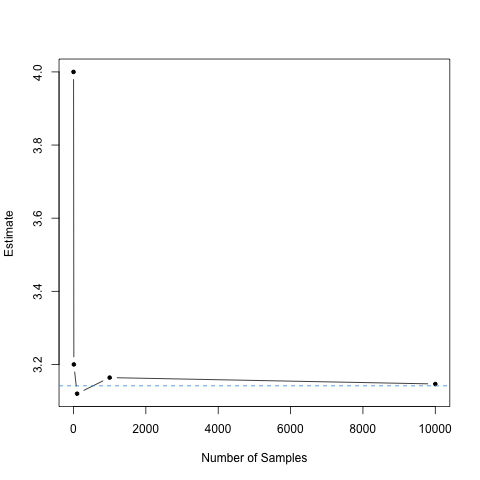
We can also plot the estimates, and compare them to the value of \(\pi\) contained in R, which is accessible through pi and is denoted by the dashed horizontal line.
plot(c(1,10,100,1000, 10000),
     pi_vec,
     type ='b',
     pch = 20,
     xlab = "Number of Samples",
     ylab = "Estimate")
abline(h = pi, col = 4, lty = 2)
Suppose we want to do the same in C++. We can write the C++ code in a seperate file with a .cpp, then call it within R using the sourceCpp() function provided in the Rcpp package. For completeness, the C++ source code contained in the file pi.cpp is as follows:
Loading the function into R is as simple as calling sourceCpp():
sourceCpp("pi.cpp")
We can now run the function:
pi_cpp(10000)
[1] 3.1368
Finally, let’s compare it with the R implementation using microbencmark:
results <- microbenchmark(pi_R(1e6), pi_cpp(1e6))
summary(results)
           expr       min        lq      mean    median       uq      max neval
1   pi_R(1e+06) 13.200319 13.955457 14.982102 14.191412 14.81519 26.64340   100
2 pi_cpp(1e+06)  8.339154  8.391716  8.683018  8.419248  8.49766 16.95912   100
In addition: Warning message:
In microbenchmark(pi_R(1e+06), pi_cpp(1e+06)) :
  less accurate nanosecond times to avoid potential integer overflows
The C++ version is about twice as fast as the R version using 1e6 samples.