Project: Conway’s Game of Life - CPU vs GPU Implementation#
Resource Files#
The job submission scripts specifically configured for use on the University of Exeter ISCA HPC system are available here.
General-purpose job submission scripts, which can serve as a starting point for use on other HPC systems (with minor modifications required for this course), are available here.
The Python scripts used in this course can be downloaded here.
All supplementary files required for the course are available here.
The presentation slides for this course can be accessed here.
Overview#
In this project, we are going to see implementations of Conway’s Game of Life, a classic cellular automaton in three ways: a pure python approach (to run on the CPU), a vectorised approach using NumPy (to run on the CPU) and then using CuPy (to run on the GPU). We’ll also visualise the evolution of the Game of Life grid to see the computation in action.
What is Conway’s Game of Life?#
It’s a zero-player game devised by John Conway, where you have a grid of cells that live or die based on a few simple rules:
Each cell can be “alive” (1) or “dead” (0).
At each time step (generation), the following rules apply to every cell simultaneously:
Any live cell with fewer than 2 live neighbours dies (underpopulation).
Any live cell with 2 or 3 live neighbours lives on to the next generation (survival).
Any live cell with more than 3 live neighbours dies (overpopulation).
Any dead cell with exactly 3 live neighbours becomes a live cell (reproduction).
Neighbours are the 8 cells touching a given cell horizontally, vertically, or diagonally.
From these simple rules emerges a lot of interesting behaviour – stable patterns, oscillators, spaceships (patterns that move), etc. It’s a good example of a grid-based simulation that can benefit from parallel computation because the state of each cell for the next generation can be computed independently (based on the current generation).
Visualisation of Game of Life#
To make this project more visually engaging, below is an animated GIF showing an example of a Game of Life simulation starting from a random initial configuration. White pixels represent live cells, and black pixels represent dead cells. You can see patterns forming, moving, and changing over time: An example evolution of Conway’s Game of Life over a few generations (white = alive, black = dead). The animation demonstrates how random initial clusters of cells can evolve into interesting patterns. Notice some cells blink on and off or form moving patterns.
The animation shows 50 timesteps on a 100x100 grid.
Implementations#
All of the implementation for the three different versions (Pure Python, NumPy and CuPy) are contained within the .py located at game_of_life.py within the scripts folder that can be downloaded at the top of this page.
To run the different versions of the code, you can use:
Naïve Python Version
python game_of_life.py run_life_naive --size 100 --timesteps 50
which will produce a file called game_of_life_naive.gif.
CPU-Vectorized Version
python game_of_life.py run_life_numpy --size 100 --timesteps 50
which will produce a file called game_of_life_cpu.gif.
GPU-Accelerated Version
python game_of_life.py run_life_cupy --size 100 --timesteps 50
which will produce a file called game_of_life_gpu.gif.
Naive Implementation#
The core computation that is being performed for the naive implementation is:
def life_step_naive(grid: np.ndarray) -> np.ndarray:
    N, M = grid.shape
    new = np.zeros((N, M), dtype=int)
    for i in range(N):
        for j in range(M):
            cnt = 0
            for di in (-1, 0, 1):
                for dj in (-1, 0, 1):
                    if di == 0 and dj == 0:
                        continue
                    ni, nj = (i + di) % N, (j + dj) % M
                    cnt += grid[ni, nj]
            if grid[i, j] == 1:
                new[i, j] = 1 if (cnt == 2 or cnt == 3) else 0
            else:
                new[i, j] = 1 if (cnt == 3) else 0
    return new

def simulate_life_naive(N: int, timesteps: int, p_alive: float = 0.2):
    grid = np.random.choice([0, 1], size=(N, N), p=[1-p_alive, p_alive])
    history = []
    for _ in range(timesteps):
        history.append(grid.copy())
        grid = life_step_naive(grid)
    return history
Explanation#
There are a number of different reasons that the naive implementation runs slow, including:
Nested Python Loops: Instead of eight
np.rollcalls and onenp.where, we make two loops overi, j(10^4 iterations) and two more loops overdi, dj(9 checks each), for roughly 9x10^4 Python level operation per step.Manual edge-wrapping logic: Branching (
if ni < 0 … elif …) for each neighbour check, instead of the single fast shift thatnp.rolldoes in C.Per-cell rule application The game of life rule is applied with Python
if/elseinstead of the single vectorised Boolean mask.Rebuilding a new NumPy array element-by-element: writing into
new_grid[i, j]in Python is orders of magnitude slower than one-shotnp.where.
Together, these overheads make this version run very slow, particularly as N begins to increase, and would not leverage any low-level C loops or GPU acceleration.
CPU-Vectorised Implementation#
def life_step_numpy(grid: np.ndarray) -> np.ndarray:
    neighbours = (
        np.roll(np.roll(grid, 1, axis=0), 1, axis=1) +
        np.roll(np.roll(grid, 1, axis=0), -1, axis=1) +
        np.roll(np.roll(grid, -1, axis=0), 1, axis=1) +
        np.roll(np.roll(grid, -1, axis=0), -1, axis=1) +
        np.roll(grid, 1, axis=0) +
        np.roll(grid, -1, axis=0) +
        np.roll(grid, 1, axis=1) +
        np.roll(grid, -1, axis=1)
    )
    return np.where((neighbours == 3) | ((grid == 1) & (neighbours == 2)), 1, 0)


def simulate_life_numpy(N: int, timesteps: int, p_alive: float = 0.2):
    grid = np.random.choice([0, 1], size=(N, N), p=[1-p_alive, p_alive])
    history = []
    for _ in range(timesteps):
        history.append(grid.copy())
        grid = life_step_numpy(grid)
    return history
Explanation#
From Per-Cell Loops to Whole-Array Operations#
In the naive version, every one of the NxN cells in Python was traversed within two nested loops; then, for each cell, two more loops over the offsets di and dj counted its eight neighbours by computing. (i + di) % N and (j + dj) % M in pure Python.
Cost: ~9·N² Python-level iterations per generation, including branching and modulo arithmetic.
Drawback Thousands of interpreter calls and non-contiguous memory access.
In the NumPy version, no Python loops over individual cells occur. Instead, eight calls to np.roll shift the entire grid array (up, down, left, right and on diagonals), automatically handling wrap-around in one C-level operation. Summing those eight arrays gives a full neighbour count in a single, optimised pass.
Manual if/else vs Vectorised Mask#
In the naive implementation, after counting neighbours, each cell’s fate is determined with a Python if grid[i,j] == 1: ... else: ... and assigned via new[i,j] = ....
In the NumPy implementation a single expression of (neighbours == 3) | ((grid == 1) & (neighbours == 2)) produces an NxN Boolean mask of cells alive next. Converting that mask to integers with np.where(mask, 1, 0) builds the entire next-generation grid in one C-level operation, resulting in no per-element Python overhead.
Automatic Wrap-Around vs Manual Modulo Logic#
In the naive version, every neighbour checks does:
ni = (i + di) % N
nj = (j + dj) % M
with Python-level branching and modulo arithmetic on each of the 9 checks per cell. The associated cost is thousands of modulo (%) operations and branch instructions per generation.
In the NumPy version, a single call to
np.roll(grid, shift, axis=)
automatically wraps the entire array in one C-level operation. The benefit is that all per-cell % operations and branching are eliminated, being replaced by a single optimised memory shift over the whole grid.
GPU-Accelerated Implementation#
def life_step_gpu(grid: cp.ndarray) -> cp.ndarray:
    neighbours = (
        cp.roll(cp.roll(grid, 1, axis=0), 1, axis=1) +
        cp.roll(cp.roll(grid, 1, axis=0), -1, axis=1) +
        cp.roll(cp.roll(grid, -1, axis=0), 1, axis=1) +
        cp.roll(cp.roll(grid, -1, axis=0), -1, axis=1) +
        cp.roll(grid, 1, axis=0) +
        cp.roll(grid, -1, axis=0) +
        cp.roll(grid, 1, axis=1) +
        cp.roll(grid, -1, axis=1)
    )
    return cp.where((neighbours == 3) | ((grid == 1) & (neighbours == 2)), 1, 0)


def simulate_life_cupy(N: int, timesteps: int, p_alive: float = 0.2):
    grid_gpu = (cp.random.random((N, N)) < p_alive).astype(cp.int32)
    history = []
    for _ in range(timesteps):
        history.append(cp.asnumpy(grid_gpu))
        grid_gpu = life_step_gpu(grid_gpu)
    return history
CuPy vs NumPy: What’s Changed.#
The power of CuPy lies in its near drop-in compatibility with NumPy: arrays live on the GPU, and computations run in parallel on the Device, yet the code looks almost identical.
Imports#
The first change you will need to make is to use CuPy rather than NumPy. NumPy:
import numpy as np
CuPy:
import cupy as cp
Random initialisation#
NumPy:
grid = np.random.choice([0,1], size=(N,N), p=[1-p, p])
CuPy:
grid_gpu = (cp.random.random((N,N)) < p_alive).astype(cp.int32)
Data Transfer#
CuPy:
cp.asnumpy(grid_gpu) # bring a CuPy array back to NumPy
Which to use?#
Large grids (e.g. N ≥ 500) or many timesteps: GPU’s parallel throughput outweighs kernel-launch and transfer overhead. Small grids (e.g. 10×10): GPU overhead may dominate, so you may want to stick with NumPy.
Why is this quicker?#
When a computation can be expressed as the same operation applied independently across many data elements, like counting neighbours on every cell of a large Game of Life grid, GPUs often deliver dramatic speedups compared to CPUs. This advantage stems from several architectural and compiler-related factors that we discussed earlier in the section on theory, including:
Massive Data Parallelism
CPU: A few (4–16) powerful cores optimised for sequential tasks and complex control flow.
GPU: Hundreds to thousands of simpler cores running in lock-step.
Result: A Game of Life update, which is identical work on each of N² cells, can be dispatched as thousands of parallel GPU threads, sweeping through the grid in a single kernel launch instead of looping in software.
Throughput-Oriented Design
CPU cores focus on single-thread performance (high clock speeds, deep pipelines, branch prediction).
GPU cores sacrifice single-thread speed in favour of raw arithmetic throughput and memory bandwidth across many threads.
Result: When you need to process millions of cell updates, the GPU’s aggregate arithmetic and memory bandwidth far outstrips what a CPU can deliver.
Specialised Memory Hierarchy
CPU: Large multi-level caches and direct access to system RAM.
GPU: High-bandwidth device memory (VRAM), with its own caches and shared memory for thread blocks.
Result: Once the grid is transferred to GPU memory, all subsequent neighbour-count rolls and mask evaluations occur on-device, benefiting from coalesced global reads and fast on-chip scratchpads.
Compiled GPU Kernels vs. Interpreted Loops
CPU code that uses Python loops incurs per-iteration interpreter overhead. Even NumPy’s C loops run on a single core.
GPU kernels compiled ahead of time by NVCC or generated at runtime execute the same inner logic entirely in device code without returning to Python between elements.
Result: You replace thousands of Python bytecode dispatches or even C-loop iterations with just a few kernel launches and a handful of device-resident function calls.
In summary,, for problems like Conway’s Game of Life, where the same simple computation is applied independently across a large array, GPUs excel by running thousands of data-parallel threads in hardware, backed by specialised memory systems and aggressive compiler optimisations. Offloading to the GPU transforms an O(N²) loop of Python or C iterations into just a handful of highly parallel kernel launches, yielding orders-of-magnitude speedups on sufficiently large grids.
How much quicker?#
Each implementation exhibits a different overall runtime, as you have probably noticed when running them from the command line. We can use the built-in UNIX command line tool time to measure the time that is taken to run the code. The time command is a simple profiler that measures how long a given program takes to run. It provides three primary metrics, including:
real: The “wall-clock” time elapsed from start to finish (i.e. actual elapsed time).
user: CPU time spent in user-mode (your programs own computations)
sys: CPU time spent in kernel mode (system calls on behalf of your program).
Framework Comparison on Each Machine
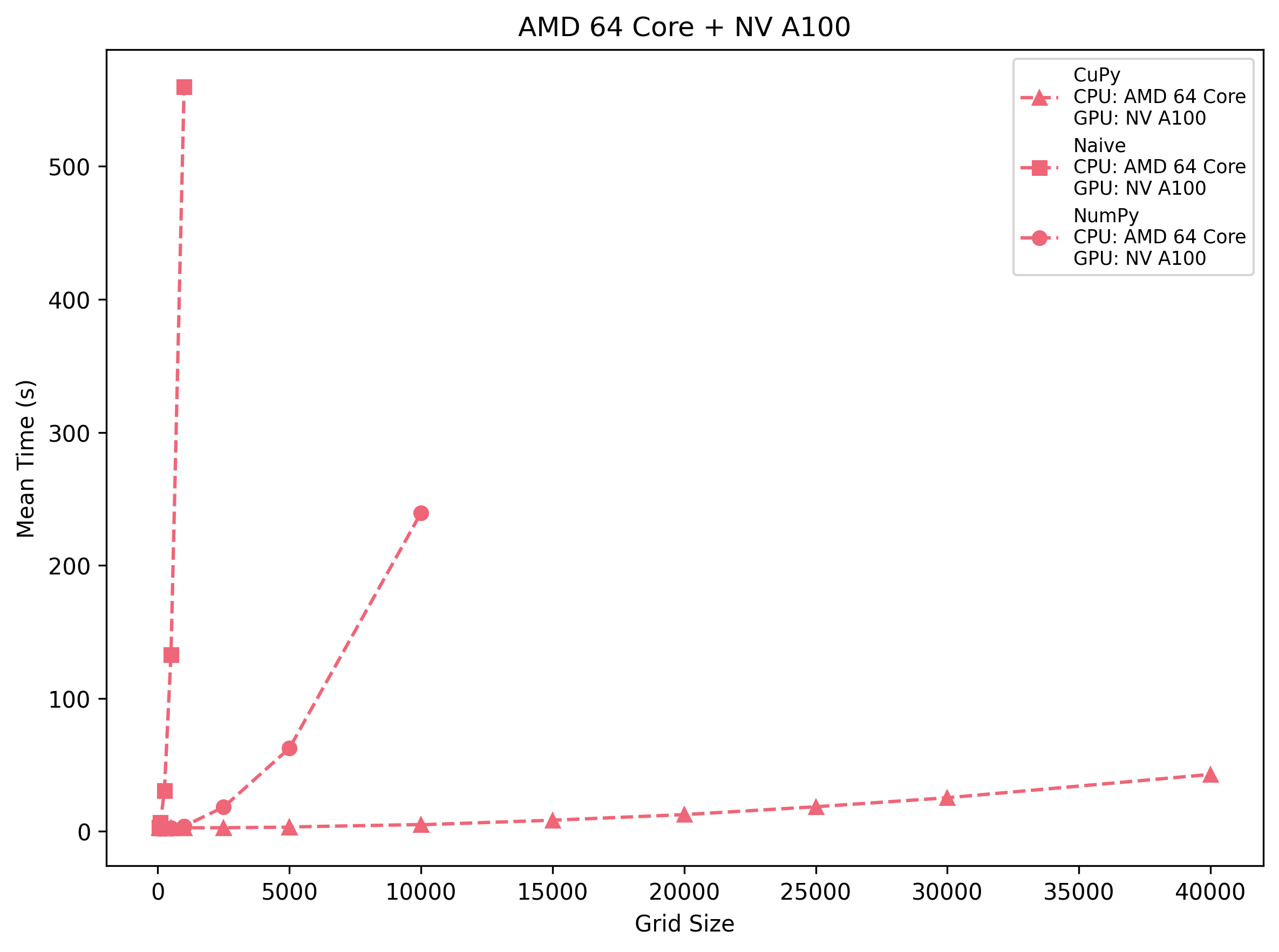
AMD 64-Core + NV A100
CuPy pays a ~2.7 s launch cost but then stays nearly flat up to 2.5 k cells, after which it grows to ~42.9 s at 40 k. NumPy starts faster on very small grids (∼2.1 s at 250) but surpasses CuPy by 500–1 k cells and balloons to ~239 s at 10 k. The naive triple loop is usable only below 250×250—beyond that you hit >130 s at 500 and ~560 s at 1 k.
Takeaway: On the A100, CuPy becomes the clear winner past ~600 cells per side. NumPy is fine for a few hundred but uncompetitive beyond 1 k, and pure Python loops become unusable quickly.
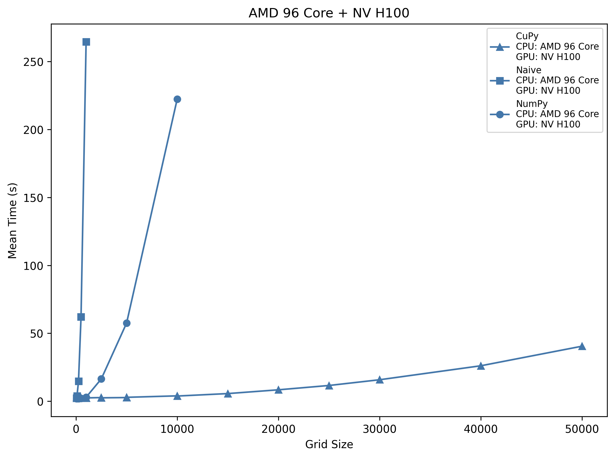
AMD 96-Core + NV H100
CuPy’s overhead shrinks slightly (~2.5 s) and its growth to ~26.1 s at 40 k is gentler than on the A100. NumPy remains sub-3 s until 1 k but then rises to ~222 s at 10 k, faster than the 64-core host only for the very largest sizes. Naive loops on this 96-core machine still hit ~62 s at 500 and ~265 s at 1 k.
Takeaway: The H100 host’s extra cores give NumPy ~10–20% speed-up over the 64-core EPYC, but CuPy is still >8× faster than NumPy past 2 k, and >100× faster than naive loops at 1 k.
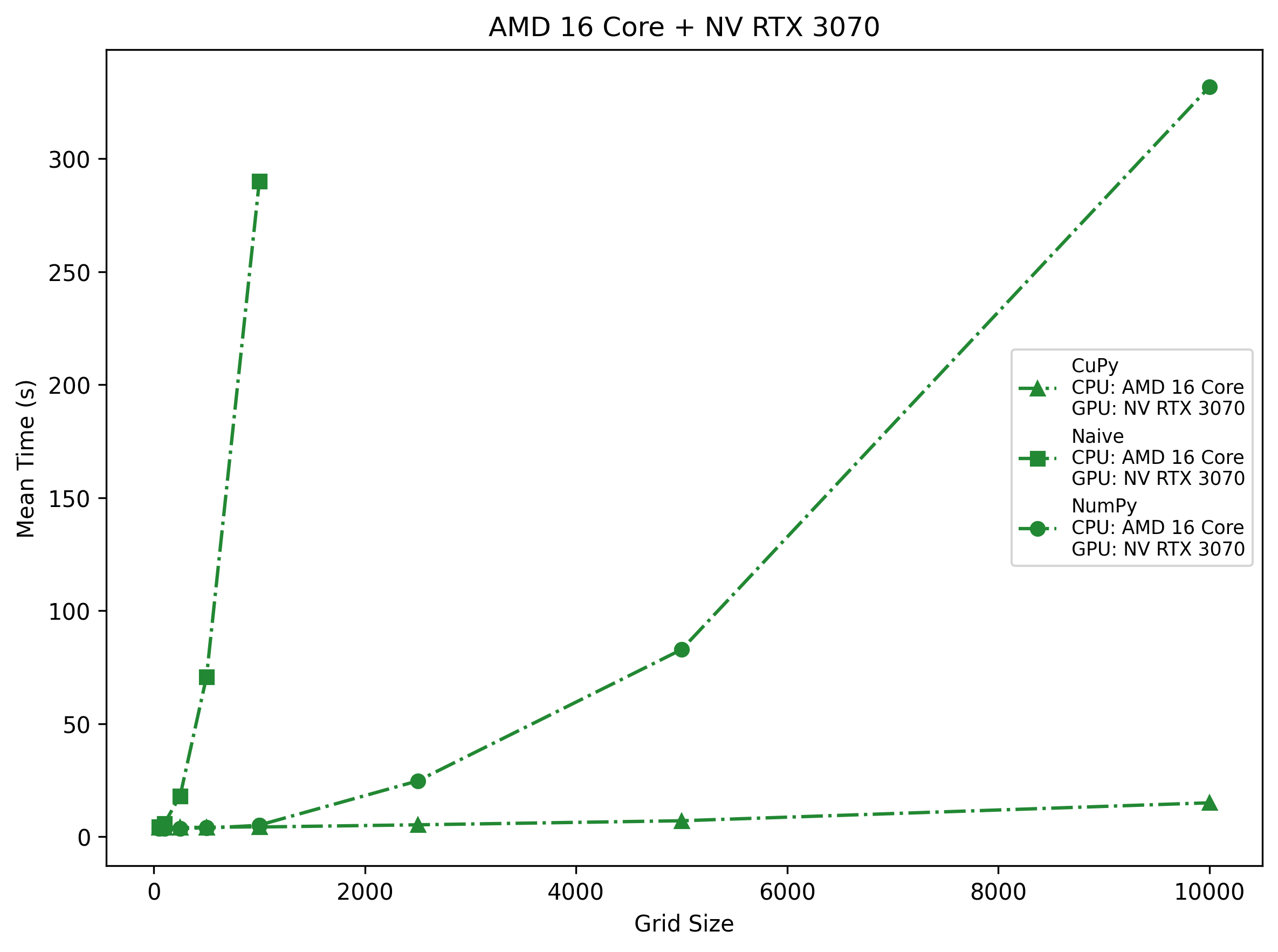
AMD 16-Core + NV RTX 3070
The midrange RTX 3070 shows ~3.9 s overhead up to 1 k, then climbs to ~14.2 s at 10 k—still well below NumPy’s ~331.9 s at 10 k on 16 cores. However, because it has fewer SMs, the plateau appears earlier (around 5 k). Naive loops cross ~70 s at 500 and ~290 s at 1 k, so even here Python loops are unusable.
Takeaway: On consumer-grade hardware, CuPy wins beyond ~400 cells per side; NumPy can handle a few thousand but then spirals into minutes, and naive loops are only for toy problems.
Machine Comparison on Each Framework
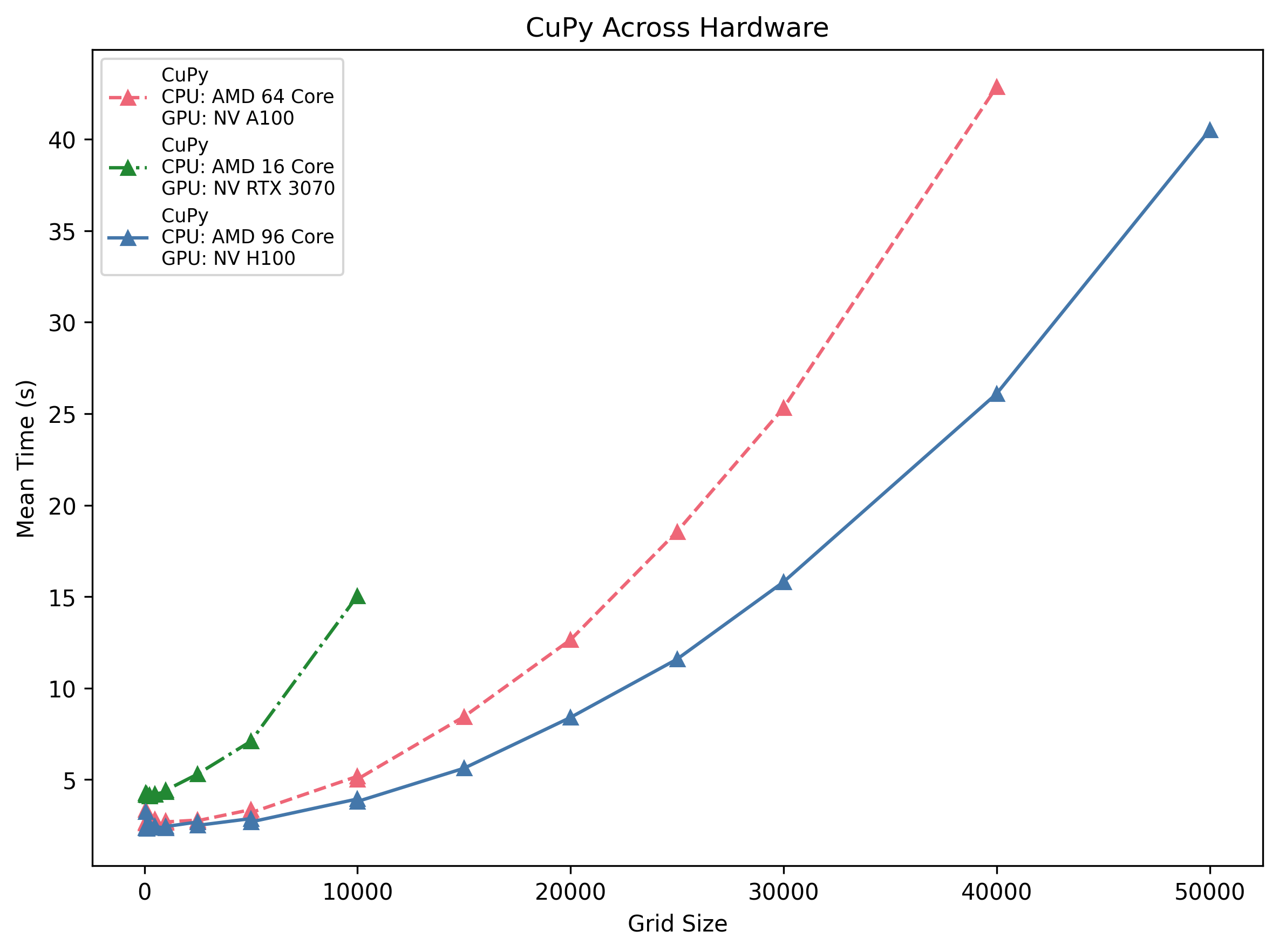
CuPy Across Hardware
All three GPUs show a ~2.5–4 s startup cost. The H100 host is the fastest at scale (∼26 s @40 k), followed by the A100 (∼43 s) and the RTX 3070 (∼14 s @10 k). Their scaling is roughly quadratic in grid side length, but the higher-end cards pull away as problem size grows.
Insight: If your grid exceeds ~1 k per side, even a midrange 3070 will beat any CPU—just be mindful of that initial launch overhead.
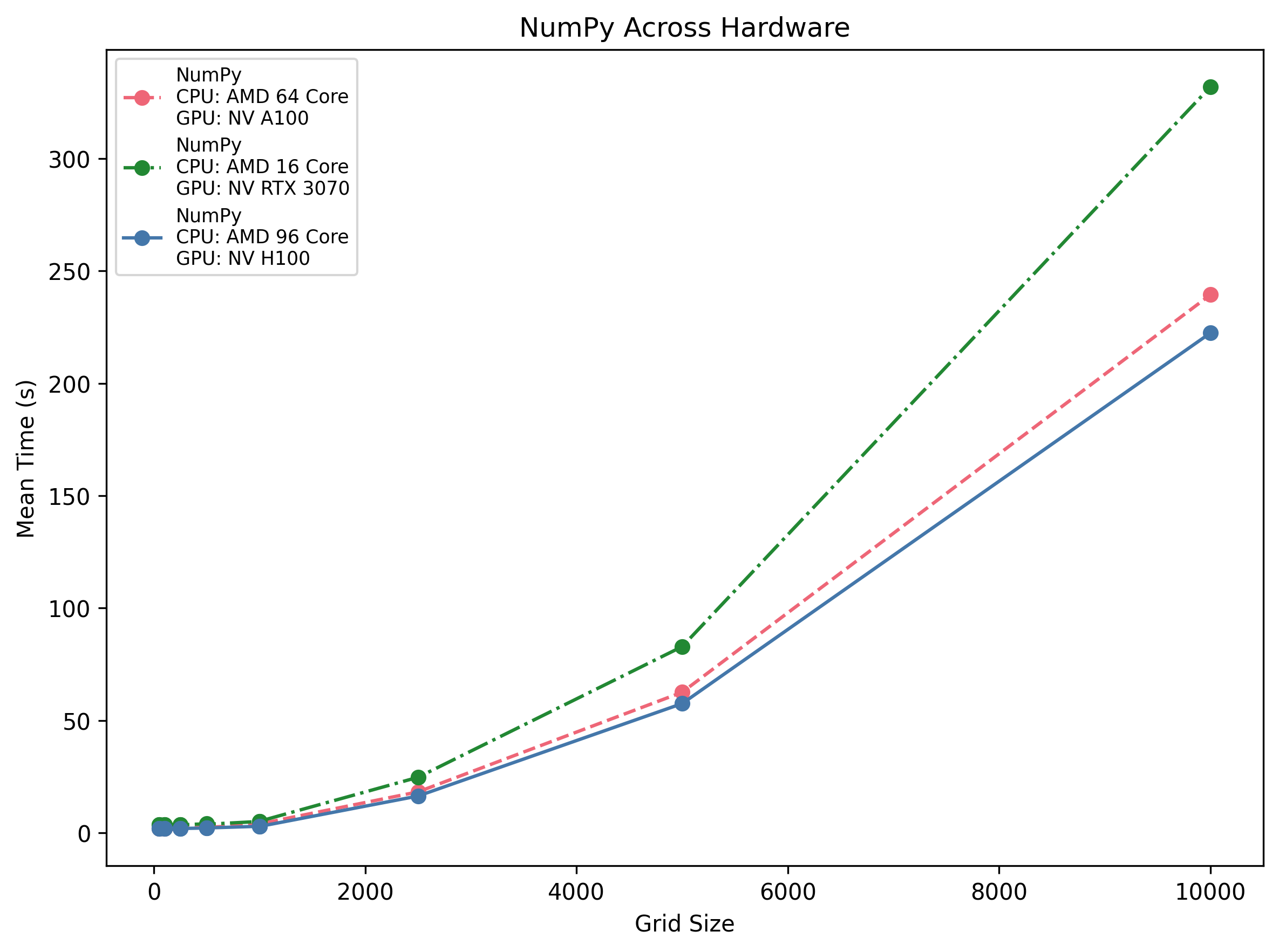
NumPy Across Hardware
Vectorised CPU performance scales with core count: the 96-core H100 host does ~2.9 s @1 k and ~222 s @10 k, the 64-core EPYC hits ~3.9 s @1 k and ~239 s @10 k, and the 16-core Ryzen only ~5.2 s @1 k but then ~332 s @10 k.
Insight: Doubling cores cuts runtime roughly in half, but you never beat the GPU’s parallelism for large areas.
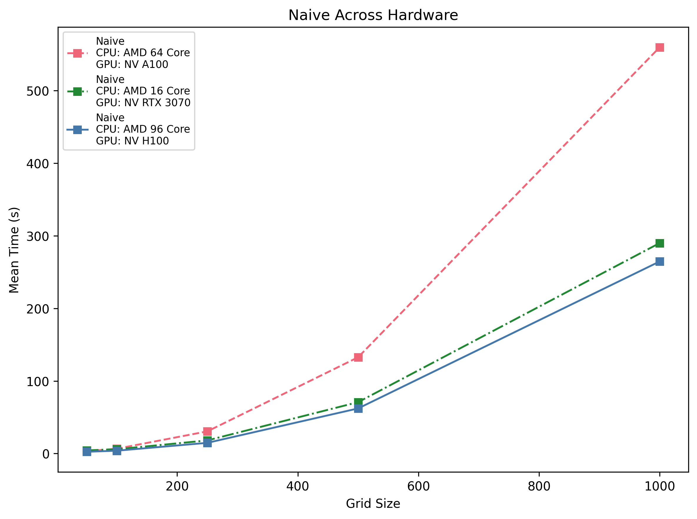
Naive Across Hardware
Pure Python loops are orders of magnitude slower across the board: even on the H100 host the run times are ~62 s @500 and ~265 s @1 k. On the 3070 machine it’s ~70 s @500, and on the A100 host ~132 s @500.
Insight: Triple-nested loops simply don’t scale. They’re only viable for extremely small toy problems (<250×250).
Inter-Machine-Framework Comparison
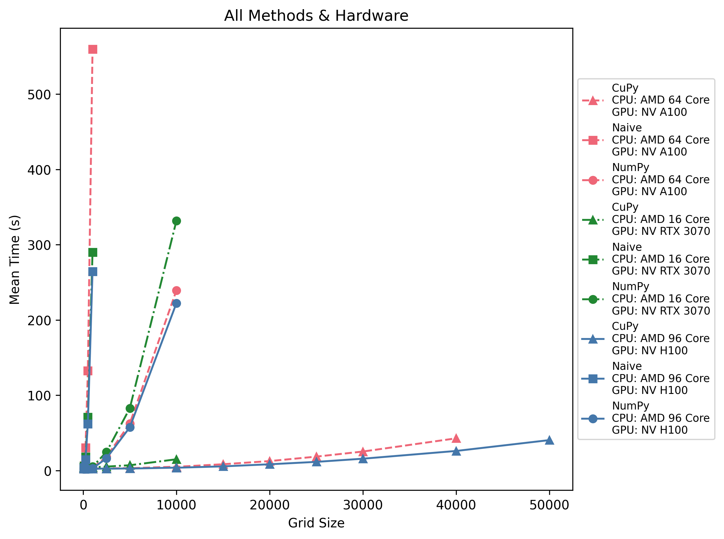
All Methods & Hardware
Across all three machines, CuPy becomes faster than NumPy at roughly 500–1 k grid size, while naive loops are unusable past ~250. GPU dispatch overhead (~3 s) means tiny grids still favor NumPy or CPU, but anything beyond a few thousand cells per side is best done with CuPy on a modern accelerator.
Exercise: Generate and Visualise Game-of-Life Performance Data#
In this exercise, you will:
Run a SLURM job to generate timing data for Conway’s Game of Life on your platform.
Modify or extend the provided plotting script to visualize that data.
Interpret and discuss the performance trends you observe.
Note: This is an open-ended assignment—feel free to experiment with new plot styles, additional metrics, or entirely custom analyses.
Generate Timing Data#
Open the
game_of_life.slurmslurm script.Edit the script to match your cluster’s configuration (e.g. partition, module loads).
Submit the job:
sbatch game_of_life.slurm
After completion, you’ll find CSV files in data/ named like:
gol_timings_<MachineName>_<Implementation>_ts100.csv
Review and Adapt the Starter Code#
The file content/game_of_life_create_plots.py contains:
CSV loading logic (from
data/)Function for:
Per-machine “Framework vs Grid Size” plots
Per-framework “Machine Comparison” plots
Combined “All Methods & Hardware” overlay
You may wish to use them as they are, or you could:
Modify these functions (styles, scales, annotations).
Rewrite your own plotting script or Jupyter notebook.
Visualisations#
Visualisations you could create include:
Framework Comparison on Each Machine: One figure per machine (e.g. A100, H100, RTX 3070) showing NumPy, Naive, CuPy timings vs. grid size.
Machine Comparison on Each Framework: One figure per framework, overlaying the three machines.
All Methods & Hardware: A combined overlay with all nine curves in a single plot.
Any other plot you can think of!
Potential Enhancements#
To extend the work you are done, you could:
Calculate Speedup ratios (e.g. CPU_time / GPU_time).
Efficiency metrics such as time per cell or memory throughput.
Annotations marking crossover points or “break-even” grid sizes.
Interactive or animated plots (e.g. showing performance evolution as grid size increases).
Finer Grained Timing Information#
Our next step is to quantify those differences by measuring exactly how long each stage takes (pure computation, data transfers, grid initialisation, etc.) and to pinpoint where the bulk of the time is spent. The following section will address these questions by introducing profiling techniques.