Profiling and Optimisation of CPU and GPU Code

Learning Objectives

By the end of this section, learners will be able to:

• Interpret GPU profiling outputs, including kernel execution times, CUDA API calls, and memory transfer operations.

• Compare the performance of naive Python, NumPy, and CuPy implementations across different problem sizes.

• Identify performance bottlenecks such as excessive Python loops, implicit synchronisations (e.g. cudaFree), and frequent small memory transfers.

• Distinguish between compute-bound and memory-bound workloads by analyzing profiling data.

• Explain the impact of kernel launch overhead, device-to-device memory copies, and synchronisation points on GPU performance.

• Recognize when GPU acceleration provides benefits over CPU execution and determine crossover points where GPU use becomes advantageous.

• Propose optimisation strategies for both CPU (e.g., vectorisation, efficient libraries, multiprocessing) and GPU (e.g., minimising data transfers, kernel fusion, asynchronous overlap, coalesced memory access).

• Apply profiling insights to guide real-world optimisation decisions in scientific or machine learning workflows.

Resource Files

The job submission scripts specifically configured for use on the University of Exeter ISCA HPC system are available here.

General-purpose job submission scripts, which can serve as a starting point for use on other HPC systems (with minor modifications required for this course), are available here.

The Python scripts used in this course can be downloaded here.

All supplementary files required for the course are available here.

The presentation slides for this course can be accessed here.

Overview

Writing code is the first problem, but generally, the second is optimising code for performance, an equally important skill, especially in GPU computing. Before optimising, you need to know where the time is being spent, which is where profiling comes in. Profiling means measuring the performance characteristics of your program, typically which parts of the code consume the most time or resources.

Profiling Python Code with cPython (CPU)

Python has a built-in profiler called cPython. It can help you find which functions are taking up the most time in your program. This is key before you go into GPU acceleration; sometimes, you might find bottlenecks in places you didn’t expect or identify parts of the code that would benefit the most from being moved to the GPU.

How to use cProfile

You can make use of cProfile via the command line: python -m cProfile -o profile_results.pstats myscript.py, which will run myscript.py under the profiler and output stats to a file. In the following examples we will instead call cProfile directly within our scripts, and use the pstat library to create immediate summaries.

import cProfile
import pstats
import numpy as np

# ─────────────────────────────────────────────────────────────────────────────
# 1) Naïve Game of Life implementation
# ─────────────────────────────────────────────────────────────────────────────

def life_step_naive(grid: np.ndarray) -> np.ndarray:
    N, M = grid.shape
    new = np.zeros((N, M), dtype=int)
    for i in range(N):
        for j in range(M):
            cnt = 0
            for di in (-1, 0, 1):
                for dj in (-1, 0, 1):
                    if di == 0 and dj == 0:
                        continue
                    ni, nj = (i + di) % N, (j + dj) % M
                    cnt += grid[ni, nj]
            if grid[i, j] == 1:
                new[i, j] = 1 if (cnt == 2 or cnt == 3) else 0
            else:
                new[i, j] = 1 if (cnt == 3) else 0
    return new

def simulate_life_naive(N: int, timesteps: int, p_alive: float = 0.2):
    grid = np.random.choice([0, 1], size=(N, N), p=[1-p_alive, p_alive])
    history = []
    for _ in range(timesteps):
        history.append(grid.copy())
        grid = life_step_naive(grid)
    return history

# ─────────────────────────────────────────────────────────────────────────────
# 2) Profiling using cProfile
# ─────────────────────────────────────────────────────────────────────────────

N = 200
STEPS = 100
P_ALIVE = 0.2

profiler = cProfile.Profile()
profiler.enable()                  # ── start profiling ────────────────

# Run the full naïve simulation
simulate_life_naive(N=N, timesteps=STEPS, p_alive=P_ALIVE)

profiler.disable()                 # ── stop profiling ─────────────────
profiler.dump_file("naive.pstat")  # ── save output ────────────────────

stats = pstats.Stats(profiler).sort_stats('cumtime')
stats.print_stats(10)              # print top 10 functions by cumulative time

Interpreting cProfile output: When you print stats, you’ll see a table with columns including:

• ncalls: number of calls to the function

• tottime: total time spent in the function (excluding sub-function calls)

• cumtime: cumulative time spent in the function includes sub-functions

• The function name

   ncalls  tottime  percall  cumtime  percall filename:lineno(function)
        1    0.034    0.034    4.312    4.312 4263274180.py:27(simulate_life_naive)
      100    4.147    0.041    4.150    0.041 4263274180.py:9(life_step_naive)
... (other functions)

Therefore in the above table ncalls (100) tells you life_step_naive was invoked 100 times; tottime (4.147 s) is the time spent inside life_step_naive itself, excluding any functions it calls; cumtime (4.150 s) is the total cumulative time in life_step_naive plus any sub-calls it makes. In this example, life_step_naive spent about 4.147 s in its own Python loops, and an extra ~0.003 s in whatever minor sub-calls it did (array indexing, % operations, etc.), for a total of 4.150 s. The per-call columns are simply tottime/ncalls and cumtime/ncalls, and the single call to simulate_life_naive shows its cumulative 4.312 s includes all the 100 naive steps plus the list-append overhead.

Visualising the Output with Snakeviz

Snakeviz is a separate tool that we can use to analyse the output of cProfile. Snakeviz is a stand-alone tool available through PyPI. We can install it with

poetry add snakeviz

We can use it to visualise a cProfile output such as the one generated from the above snippet

poetry run snakeviz naive.pstat

which launches an interactive webapp which we can use to explore the profiling timings.

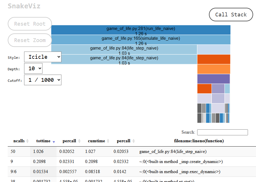
Finding Bottlenecks

To pinpoint where your code spends most of its time, look at the cumulative time (cumtime) column in the profiler report. This shows the total time in a function plus all of its sub-calls. A high total time (tottime) means that the function’s own Python code is heavy, whereas a large gap between cumtime and tottime reveals significant work in any functions it invokes (array indexing, modulo ops, etc.).

In our naive Game of Life example:

• life_step_naive is called 100 times, with tottime ≈ 4.147 s and cumtime ≈ 4.150 s.

  • Almost all the work is in its own nested loops and per-cell logic.

  • Only a few milliseconds are spent in its sub-calls (grid indexing, % arithmetic).

• simulate_life_naive appears once with cumtime ≈ 4.312 s, which covers the single Python loop plus all 100 calls to life_step_naive.

Once you’ve identified the culprit:

• If you have high tottime in a Python function, you may want to consider consider vectorising inner loops (e.g. switch to NumPy’s np.roll + np.where) or using a compiled extension.

• If you have heavy external calls under your cumtime, then you may want to explore hardware acceleration (e.g. GPU via CuPy) or more efficient algorithms.

Profiling the CPU-Vectorised Implementation using NumPy.

import cProfile
import pstats
import numpy as np

# ─────────────────────────────────────────────────────────────────────────────
# 1) NumPy Game of Life implementation
# ─────────────────────────────────────────────────────────────────────────────

def life_step_numpy(grid: np.ndarray) -> np.ndarray:
    neighbours = (
        np.roll(np.roll(grid, 1, axis=0), 1, axis=1) +
        np.roll(np.roll(grid, 1, axis=0), -1, axis=1) +
        np.roll(np.roll(grid, -1, axis=0), 1, axis=1) +
        np.roll(np.roll(grid, -1, axis=0), -1, axis=1) +
        np.roll(grid, 1, axis=0) +
        np.roll(grid, -1, axis=0) +
        np.roll(grid, 1, axis=1) +
        np.roll(grid, -1, axis=1)
    )
    return np.where((neighbours == 3) | ((grid == 1) & (neighbours == 2)), 1, 0)

def simulate_life_numpy(N: int, timesteps: int, p_alive: float = 0.2):
    grid = np.random.choice([0, 1], size=(N, N), p=[1-p_alive, p_alive])
    history = []
    for _ in range(timesteps):
        history.append(grid.copy())
        grid = life_step_numpy(grid)
    return history

# ─────────────────────────────────────────────────────────────────────────────
# 2) Profiling using cProfile
# ─────────────────────────────────────────────────────────────────────────────

N = 200
STEPS = 100
P_ALIVE = 0.2

profiler = cProfile.Profile()
profiler.enable()  # ── start profiling ────────────────────────

# Run the full NumPy-based simulation
simulate_life_numpy(N=N, timesteps=STEPS, p_alive=P_ALIVE)

profiler.disable()  # ── stop profiling ─────────────────────────
profiler.dump_file('numpy.pstat')  # ── save output ─────────────────────────

stats = (
    pstats.Stats(profiler)
          .strip_dirs()                  # remove full paths
          .sort_stats('cumtime')         # sort by cumulative time
)
# show only the NumPy functions in the report
stats.print_stats(r"life_step_numpy|simulate_life_numpy")

ncalls  tottime  percall  cumtime  percall filename:lineno(function)
   100    0.028    0.000    0.055    0.001 2865127924.py:9(life_step_numpy)
     1    0.000    0.000    0.011    0.011 2865127924.py:22(simulate_life_numpy)

Interpreting the Results

life_step_numpy ncalls = 100: called once per generation for 100 generations, the same as before. tottime ≈ 0.028 s: time spent in the Python-level wrapper (the eight np.roll calls and the one np.where, excluding the internal C work. cumtime ≈ 0.055 s: includes both the Python-level overhead and the time spent inside NumPy’s compiled code (rolling, adding, masking, etc.) simulate_life_numpy ncalls = 1: the top-level driver is run once. cumtime ≈ 0.011 s: covers grid initialisation, 100 calls to life_step_numpy, and the history list appends.

Why is it so much faster than the naive version?

• Bulk C-level operations

  • The eight np.roll shifts and the single np.where are all implemented in optimised C loops.

  • cProfile only attributes a few milliseconds to Python itself because the heavy lifting happens outside Python’s interpreter.

• Minimal Python overhead

  • We pay one Python-level call per generation (100 calls total) versus hundreds of thousands of Python-loop iterations in the naive version.

  • That drops the Python-layer tottime from ~4s (naive) to ~0.03s (NumPy)

• Cache and vector-friendly memory access

  • NumPy works on large contiguous buffers, so the CPU prefetches data and applies vector instructions.

  • The naïve per-cell modulo arithmetic and scattered indexing defeat those hardware optimisations.

Overall, by moving the neighbour counting and rule application into a few large NumPy calls, we cut down Python‐level time from over 4 seconds to under 0.1 seconds for 100 generations on a 200×200 grid.

Profiling GPU Code with NVIDIA Nsight Systems

When we involve GPUs, cProfile alone isn’t enough. cProfile will tell us about the Python side, but we also need to know what’s happening on the GPU. Does the GPU spend most of its time computing, or is it idle while waiting for data? Are there a few kernel launches that take a long time or many tiny kernel launches?

NVIDIA Nsight Systems is a profiler for GPU applications that provides a timeline of CPU and GPU activity. It can show:

• When your code launched GPU kernels and how long they ran

• GPU memory transfers between host and device

• CPU-side functions as well (to correlate CPU and GPU)

Using Nsight Systems

Nsight Systems can be used via a GUI or command line. On clusters, you might use the CLI, assuming it’s installed.

You will need to run your script under Nsight:

nsys profile -o profile_report python my_gpu_script.py

This will run my_gpu_script.py and record profiling data into a data file with the extension .nsys-rep, creating in the above case the file profile_report.nsys-rep. The file can then be analysed with the following command:

nsys stats profile_report.nsys-rep

An example .nsys-rep file has been included within the GitHub Repo for you to try the command with, at the filepath files/profiling/example_data_file.nsys-rep. We will discuss the contents of the file in the section “Example Output” after discussing the necessary code changes to generate the file.

Code Changes

To get the fine-tuned profiling, we also need to make some changes to the code. A new version of Conway’s Game of Life has been created and is located in game_of_life_profiled.py, where additional imports are needed:

from cupyx.profiler import time_range  
from cupy.cuda import profiler

We then also need to decorate all the core functions we are interested in with a @time_range() decorator, for example:

@time_range()
def life_step_numpy():

@time_range()
def life_step_gpu():

@time_range()
def life_step_naive():

Finally we also need to start and stop the profiler, whcih is done with:

def run_life_cupy():
    if args.profile_gpu:
        profiler.start()

    history = simulate_life_cupy()

    if args.profile_gpu:
        profiler.stop()

The final change that needs to be made is to change the manner in which the Python code is called within the .slurm script using:

nsys profile --sample=none --trace=cuda,nvtx -o ../output/${SLURM_JOB_NAME}_${SLURM_JOB_ID}_exp_report -- poetry run game_of_life_experiment_profiled --profile-gpu --profile-cpu

Unfortunately, you can’t call the Python script itself as we did before as the Python interpreter obfuscates the profiler, and so there is a need to instead define a new entry point and call that to run the complete experiment run.

Together these are all the changes that are needed to create the data file and be able to understand better how the code is performing and where there is potential for further improvements through optimisation.

Example Output Grid Sizes 10, 25, 50, 100 Across Naive, NumPy, CuPy

When you run the command nsys stats on a .nsys-rep file it will generate text report of the profiling that was conducted. An example of the output producded is located at files/profiling/example_nsys_stats_output.txt, but you can run it for yourself with the command:

nsys stats files/profiling/example_data_file.nsys-rep

The following subsections detail the different components of the report generated.

NVTX Range Summary

The NVTX ranges bracket your Python/CuPy functins.

Time (%)	Total Time (ns)	Instances	Avg (ns)	Med (ns)	Min (ns)	Max (ns)	StdDev (ns)	Style	Range
36.6	8 535 674 999	12	711 306 249.9	337 956 117.5	32 066 518	2 154 888 540	879 481 300.4	PushPop	:simulate_life_naive
36.0	8 398 662 776	1200	6 998 885.6	3 274 825.5	208 959	21 511 028	8 419 478.3	PushPop	:life_step_naive
20.0	4 671 705 906	12	389 308 825.5	386 720 513.0	377 014 681	414 862 062	11 356 633.9	PushPop	:simulate_life_cupy
5.5	1 284 742 952	1200	1 070 619.1	934 097.0	894 127	12 411 105	1 001 792.4	PushPop	:life_step_gpu
1.2	276 921 198	12	23 076 766.5	22 136 591.0	20 319 042	27 672 011	2 828 715.6	PushPop	:simulate_life_numpy
0.6	144 652 945	1200	120 544.1	115 209.5	93 330	320 779	28 252.5	PushPop	:life_step_numpy

Over 72% of time sits in the naive Python loops (simulate_life_naive and life_step_naive), while the GPU vectorised step (life_step_gpu) only accounts for ~5.5%. Interesting in this context NumPy is faster than the CuPy code. The grid sizes used were [10, 25, 50, 100].

CUDA API Summary

Time (%)	Total Time (ns)	Num Calls	Avg (ns)	Med (ns)	Min (ns)	Max (ns)	StdDev (ns)	Name
86.4	1 560 619 502	60	26 010 325.0	210.0	110	137 306 387	52 472 498.8	cudaFree
6.9	125 243 240	38 436	3 258.5	2 920.0	2 280	71 249	962.6	cuLaunchKernel
2.6	46 825 640	24	1 951 068.3	1 933 764.5	1 223 737	2 732 432	721 292.2	cudaLaunchKernel
2.5	45 049 441	7 200	6 256.9	6 049.5	4 820	23 620	1 171.9	cudaMemcpyAsync
0.9	15 769 146	180	87 606.4	83 960.0	78 700	133 209	10 580.0	cuModuleLoadData
0.3	4 899 267	96	51 034.0	45 400.0	35 760	89 929	13 186.4	cuModuleUnload
0.2	3 247 650	24	135 318.8	134 505.0	103 140	201 630	24 291.5	cuLibraryUnload
0.1	2 010 781	12	167 565.1	167 964.0	163 939	168 879	1 326.3	cudaDeviceSynchronize
0.1	1 722 245	102	16 884.8	5 135.0	2 440	109 670	32 859.3	cudaMalloc
0.1	1 020 638	4 944	206.4	190.0	60	1 150	115.7	cuGetProcAddress_v2
0.0	498 689	12	41 557.4	41 500.0	34 970	45 760	3 623.0	cudaMemGetInfo
0.0	85 680	12	7 140.0	7 145.0	6 840	7 430	199.5	cudaStreamIsCapturing_v10000
0.0	17 550	24	731.3	680.0	100	1 630	599.0	cuModuleGetLoadingMode
0.0	17 110	12	1 425.8	1 415.0	1 270	1 710	140.0	cuInit

Going into the individual calls being performed within the CUDA API is outside of the scope of this course. However, this table does give a better idea of what is happening with the GPU if you require going into that detail for your optimisations. For example, cudaFree is a runtime call that releases device memory allocation. This is called in CuPy, every time a cp.ndarray (or call .get()/.astype()), to free the memory that was being used. The key part that makes this expensive is that cudaFree is a synchronous operation, so the CPU will stall until the GPU has completed this step. The actionable step we could take to reduce this is to minimise these calls. Instead of freeing every array after each iteration, we could pre-allocate a buffer once and reuse it for every step, eliminating repeated synchronisation.

GPU Kernel Execution

Time (%)	Total Time (ns)	Instances	Avg (ns)	Med (ns)	Min (ns)	Max (ns)	StdDev (ns)	Name
56.4	33 398 172	21 384	1 561.8	1 536.0	1 056	2 048	251.7	cupy_copy__int64_int64
19.9	11 784 791	8 316	1 417.1	1 440.0	1 088	1 728	158.9	cupy_add__int64_int64_int64
8.3	4 895 203	3 564	1 373.5	1 408.0	1 088	1 600	135.8	cupy_equal__int64_int_bool
3.4	2 006 447	12	167 203.9	167 233.0	166 466	167 681	412.6	void generate_seed_pseudo<rng_config<curandStateXORWOW, (curandOrdering)101>>(unsigned long long, u…)
2.8	1 655 408	1 200	1 379.5	1 440.0	1 088	1 632	154.1	cupy_bitwise_and__bool_bool_bool
2.8	1 654 728	1 200	1 378.9	1 424.5	1 056	1 600	150.5	cupy_where__bool_int_int_int64
2.8	1 639 308	1 200	1 366.1	1 408.0	1 056	1 600	149.4	cupy_bitwise_or__bool_bool_bool
2.7	1 627 787	1 200	1 356.5	1 392.0	1 056	1 664	144.8	cupy_copy__bool_bool
0.6	334 881	216	1 550.4	1 472.0	1 056	2 048	230.6	cupy_copy__int32_int32
0.2	120 513	84	1 434.7	1 456.0	1 152	1 728	153.2	cupy_add__int32_int32_int32
0.1	48 225	36	1 339.6	1 376.0	1 056	1 568	172.6	cupy_equal__int32_int_bool
0.0	18 912	12	1 576.0	1 616.0	1 344	1 856	187.6	void gen_sequenced<curandStateXORWOW, double, int, &curand_uniform_double_noargs<curandStateXORWOW>…
0.0	18 016	12	1 501.3	1 520.0	1 280	1 632	123.9	cupy_random_x_mod_1
0.0	17 600	12	1 466.7	1 504.0	1 344	1 600	102.0	cupy_less__float64_float_bool
0.0	16 512	12	1 376.0	1 536.0	1 056	1 568	211.4	cupy_copy__bool_int32

This breakdown shows that over half of all GPU kernel time is spent in the cupy_copy__int64_int64 kernel—handling bulk data movement—followed by the cupy_add__int64_int64_int64 and cupy_equal__int64_int_bool compute kernels, each taking roughly 1–1.6 µs per instance. All other kernels, including bitwise ops, conditional selects, and random‐seed generation, run in similar microsecond ranges but contribute far less overall, indicating a workload dominated by simple element‐wise copy and arithmetic operations. Highlighting that the majority of the GPU time is not being spent on computation.

GPU Memory Operations

By Time

Time (%)	Total Time (ns)	Count	Avg (ns)	Med (ns)	Min (ns)	Max (ns)	StdDev (ns)	Operation
100.0	9 124 387	7 200	1 267.3	1 312.0	960	1 472	119.7	[CUDA memcpy Device-to-Device]

By Size

Total (MB)	Count	Avg (MB)	Med (MB)	Min (MB)	Max (MB)	StdDev (MB)	Operation
186.837	7 200	0.026	0.007	0.000	0.079	0.031	[CUDA memcpy Device-to-Device]

Key Takeaways

The takeaways that we could take from this include the following:

• Python loops severely degrade performance: Over 72% of run time is in the naive implementations, so vectorisation (NumPy/CuPy) is critical.

• Implicit syncs dominate: cudaFree stalls the pipe, and so avoiding per-iteration free calls by reusing buffers is key.

• Kernel work is tiny: Each kernel takes ~1-2µs; orchestration (kernel launches + memops) is the real bottleneck.

• Memcopy patterns matter: 7200 small transfers add up, so we need to use larger batches of copies to reduce the overhead.

Example Output Grid Sizes 50, 100, 250, 500, 1000 Across Naive, NumPy, CuPy

Provided below are the same tables as above but for the Game of Life ran with grid sizes [50, 100, 250, 500, 1000].

NVTX Range Summary

Time (%)	Total Time (ns)	Instances	Avg (ns)	Med (ns)	Min (ns)	Max (ns)	StdDev (ns)	Style	Range
49.5	996 594 758 961	15	66 439 650 597.4	13 121 447 905.0	536 057 614	261 739 193 353	100 890 404 862.4	PushPop	:simulate_life_naive
49.5	996 314 582 960	1 500	664 209 722.0	131 032 064.5	5 185 001	2 635 408 984	974 949 530.9	PushPop	:life_step_naive
0.6	11 719 493 946	15	781 299 596.4	399 051 461.0	373 843 763	6 218 365 721	1 504 209 809.4	PushPop	:simulate_life_cupy
0.2	3 874 165 387	15	258 277 692.5	91 469 695.0	22 700 648	851 927 462	323 227 971.4	PushPop	:simulate_life_numpy
0.2	3 513 311 048	1 500	2 342 207.4	759 883.0	112 230	10 461 891	3 085 684.1	PushPop	:life_step_numpy
0.1	1 633 590 838	1 500	1 089 060.6	940 589.0	894 823	14 415 246	1 105 761.6	PushPop	:life_step_gpu

CUDA API Summary

Time (%)	Total Time (ns)	Num Calls	Avg (ns)	Med (ns)	Min (ns)	Max (ns)	StdDev (ns)	Name
69.2	2 541 019 787	75	33 880 263.8	230.0	120	733 443 841	96 242 335.2	cudaFree
22.5	824 537 275	30	27 484 575.8	2 278 088.5	1 190 585	495 570 646	101 802 539.0	cudaLaunchKernel
4.3	158 809 973	48 045	3 305.4	3 000.0	2 300	48 351	925.4	cuLaunchKernel
1.7	63 278 947	9 000	7 031.0	7 120.0	4 890	27 190	1 639.3	cudaMemcpyAsync
0.9	31 528 151	225	140 125.1	85 220.0	79 071	11 819 926	782 186.4	cuModuleLoadData
0.6	21 676 197	120	180 635.0	46 030.0	34 890	15 677 051	1 426 563.3	cuModuleUnload
0.4	14 435 308	15	962 353.9	5 191.0	4 730	14 363 066	3 707 195.4	cudaStreamIsCapturing_v10000
0.2	5 899 095	132	44 690.1	6 315.0	2 860	150 401	49 075.1	cudaMalloc
0.1	4 075 165	30	135 838.8	135 280.5	103 310	190 941	21 163.6	cuLibraryUnload
0.1	2 546 761	15	169 784.1	168 900.0	166 201	172 431	2 026.7	cudaDeviceSynchronize
0.0	1 251 918	6 180	202.6	180.0	60	2 020	114.9	cuGetProcAddress_v2
0.0	599 392	15	39 959.5	41 610.0	31 850	53 191	6 136.1	cudaMemGetInfo
0.0	23 950	15	1 596.7	1 460.0	1 270	3 670	592.4	cuInit
0.0	21 130	30	704.3	665.0	100	1 670	582.4	cuModuleGetLoadingMode

GPU Kernel Execution

Time (%)	Total Time (ns)	Instances	Avg (ns)	Med (ns)	Min (ns)	Max (ns)	StdDev (ns)	Name
46.6	57 042 704	26 730	2 134.0	1 824.0	1 056	7 648	1 464.2	cupy_copy__int64_int64
25.4	31 075 482	10 395	2 989.5	1 856.0	1 440	7 328	2 067.8	cupy_add__int64_int64_int64
10.6	12 926 455	4 455	2 901.6	1 760.0	1 408	7 168	2 065.3	cupy_equal__int64_int_bool
3.6	4 414 582	1 500	2 943.1	1 792.0	1 440	7 232	2 084.5	cupy_bitwise_and__bool_bool_bool
3.6	4 412 844	1 500	2 941.9	1 792.0	1 408	7 232	2 102.9	cupy_bitwise_or__bool_bool_bool
3.6	4 398 695	1 500	2 932.5	1 792.0	1 440	7 296	2 076.4	cupy_where__bool_int_int_int64
3.5	4 300 049	1 500	2 866.7	1 760.0	1 408	7 040	2 039.9	cupy_copy__bool_bool
2.1	2 535 815	15	169 054.3	167 969.0	167 297	171 872	1 744.7	void generate_seed_pseudo<rng_config<curandStateXORWOW, (curandOrdering)101>>(unsigned long long, u…)
0.5	570 464	270	2 112.8	1 664.0	1 024	7 392	1 473.7	cupy_copy__int32_int32
0.3	313 762	105	2 988.2	1 856.0	1 440	7 136	2 085.9	cupy_add__int32_int32_int32
0.1	130 881	45	2 908.5	1 792.0	1 408	7 008	2 089.1	cupy_equal__int32_int_bool
0.1	76 928	15	5 128.5	2 464.0	1 664	14 720	5 025.6	void gen_sequenced<curandStateXORWOW, double, int, &curand_uniform_double_noargs<curandStateXORWOW>…
0.0	44 896	15	2 993.1	1 856.0	1 504	6 976	2 121.2	cupy_copy__bool_int32
0.0	44 288	15	2 952.5	1 824.0	1 504	6 912	2 107.8	cupy_less__float64_float_bool
0.0	44 064	15	2 937.6	1 824.0	1 568	6 816	2 040.6	cupy_random_x_mod_1

GPU Memory Operations

By Time

Time (%)	Total Time (ns)	Count	Avg (ns)	Med (ns)	Min (ns)	Max (ns)	StdDev (ns)	Operation
100.0	29 435 086	9 000	3 270.6	1 600.0	1 248	17 888	2 406.9	[CUDA memcpy Device-to-Device]

By Size

Total (MB)	Count	Avg (MB)	Med (MB)	Min (MB)	Max (MB)	StdDev (MB)	Operation
18 957.377	9 000	2.106	0.498	0.010	7.992	3.014	[CUDA memcpy Device-to-Device]

Exercise: Undertsanding Change in Profiling Data

Now that you have seen the detailed profiling breakdowns for grid sizes [10, 25, 50, 100] and [50, 100, 250, 500, 1000], take some time to consider and answer the following:

• Scaling of Python vs Vectorised Code

  • How does the percentage of total run-time spent in the naive Python loops (simulate_life_naive + life_step_naive) change as the grid size grows?

  • At what grid size does the NumPy implementation begin to out-perform the naive Python version? And at what point does CuPy start to consistently beat NumPy?

• NumPy vs CuPy Overhead

  • For the smaller grids (10–100), NumPy was faster than CuPy, why?

  • Identify which CUDA API calls (e.g. cudaFree, cudaMalloc, cudaMemcpyAsync) dominate the overhead in the CuPy runs. How does this overhead fraction evolve for larger problem sizes?

• Kernel vs Memory-Transfer Balance

  • Examine the GPU Kernel Execution tables: what fraction of the total GPU time is spent in compute kernels (e.g. cupy_add, cupy_equal) versus simple copy kernels (e.g. cupy_copy)?

  • How does the ratio of Device-to-Device memcpy time to compute time change when moving from small to large grids?

• Impact of Implicit Synchronisations

  • The cudaFree call is synchronous and stalls the CPU; how many times is it invoked per iteration, and how much total time does it cost?

  • Propose a strategy to pre-allocate and reuse GPU buffers across iterations—how many cudaFree calls would you eliminate, and roughly how much time would this save?

• Optimisation Opportunities

  • Based on the profiling data across both grid-size ranges, what is the single biggest bottleneck you would tackle first?

  • What are some optimisations that could be used?.

• Real-World Implications

  • If this Game of Life kernel were part of a larger simulation pipeline, what lessons can you draw about when and how to offload work to the GPU?

  • At what problem size does GPU acceleration become worthwhile, and how would you detect that programmatically?

Potential Answers!

Scaling of Python vs. Vectorized Code

• Naive Python loops dominate more as the grid grows: they consume ~72% of total NVTX‐measured time for N between [10–100], and nearly 99% for N between [50–1000], showing that pure‐Python O(N²) code scales very poorly.

• NumPy is faster than the naive version even at the smallest grid (N=10) thanks to C‐level vectorisation. CuPy only begins to consistently beat NumPy once N≥250–500, where the fixed GPU launch and transfer overhead is amortised.

NumPy vs. CuPy Overhead

• For small grids (N ≤100), NumPy wins because CuPy pays extra for cudaMalloc/cudaFree, kernel launches and synchronisations on every step.

• In the CuPy runs, cudaFree alone accounts for ~86% of all CUDA API time (dropping to ~69% at larger N), followed by cuLaunchKernel. That overhead fraction shrinks slightly as compute work grows, but remains the dominant cost.

Kernel vs. Memory‐Transfer Balance

• Across both size ranges, cupy_copy__… kernels (element-wise copies) take over 50% of GPU compute time, while arithmetic kernels (cupy_add, cupy_equal) contribute ~20%. The GPU is spending more time moving data than doing math.

• The ratio of Device-to-Device memcpy to compute time decreases for larger grids: small runs saw ~9ms of memcpy vs. ~33ms of compute, whereas large runs saw ~29ms of memcpy vs. ~57ms of compute, so data‐move overhead becomes relatively less as problem size grows.

Impact of Implicit Synchronisations

• Each timestep triggers at least one cudaFree (and possibly an allocation), costing ~1.5s of sync overhead on small grids and ~2.5s on large ones. That’s >80% of API time.

• Pre-allocating two device buffers (next and current grid) and reusing them would eliminate all per-step cudaFree calls—saving roughly the entire cudaFree overhead.

Optimisation Opportunities

• First tackle the naive Python loops: replace them with NumPy or CuPy to eliminate the 70–99% NVTX‐time they consume.

• Then address the GPU syncs by pre-allocating buffers, batching kernel launches into fewer calls, and consolidating small memcopies into larger transfers.

Real‐World Implications

• In a larger pipeline you should only offload those kernels whose work (e.g. N≥250–500) justifies the overhead of transfers and launches.

• You can auto-tune by benchmarking a handful of sizes at startup and selecting CPU vs. GPU code paths based on the measured crossover point.

These answers illustrate how to interpret NVTX ranges, CUDA API tables and kernel/memop summaries to guide optimisations in a Python and CuPy workflow.

General Optimisation Strategies

Bringing everything together, some strategies include:

On the CPU side (Python):

• Vectorise Operations: We saw this with NumPy; doing things in batches is faster than Python loops.

• Use efficient libraries: If a certain computation is slow in Python, see if there is a library (NumPy, SciPy, etc) that does it in C or another language.

• Optimise algorithms: Sometimes, a better algorithm can speed things up more than any level of optimisation. For example, if you find a certain computation is N^2 in complexity and it’s slow, see if you can make it N log N or similar.

• Consider multiprocessing or parallelisation: Use multiple CPU cores (with multiprocessing or joblib or others) if appropriate.

On the GPU side:

• Minimise data transfers: Once data is on the GPU, try to do as much as possible there. Transferring large arrays back and forth every iteration will kill performance. Maybe accumulate results and transfer once at the end, or use pinned memory for faster transfers if you must.

• Kernel fusion / reducing launch overhead: Each call (like our multiple cp.roll operations) launches separate kernels. If possible, combining operations into one kernel means the GPU can do it all in one pass. Some libraries or tools do this automatically (for example, CuPy might fuse elementwise operations under the hood, and deep learning frameworks definitely fuse a lot of ops). If not, one can write a custom CUDA kernel to do more work in one go.

• Asynchronous overlap: GPUs operate asynchronously relative to the CPU. You can have the CPU queue up work and then do something else (like prepare next batch of data) while GPU is processing. Nsight can show if your CPU and GPU are overlapping or if one is waiting for the other. Ideally, you overlap communication (PCIe transfers) with computation if possible.

• Memory access patterns: This is more advanced, but if diving into custom kernel, coalesced memory access (accessing consecutive memory addresses in threads that are next to each other) is important for performance. Uncoalesced or random access can slow down even if arithmetic is small.

• Use specialised libraries: For certain tasks, libraries like cuDNN (deep neural nets), cuBLAS (linear algebra), etc., are heavily optimised. Always prefer a library call (e.g., cp.fft or cp.linalg) over writing your own, if it fits the need, because those are likely tuned for performance.