3D Temperature Diffusion Model: Bringing it all together#
Learning Objectives#
By the end of this section, learners will be able to:
Implement a naive 3D temperature diffusion model in pure Python and understand its computational limitations.
Optimise the naive implementation using NumPy for CPU execution and CuPy for GPU acceleration.
Compare runtime performance across pure Python, NumPy, and CuPy implementations using scaling plots.
Profile temperature diffusion code to identify computational bottlenecks and quantify performance improvements.
Download, summarise, and visualise real-world ocean temperature data from NetCDF files.
Use static and interactive visualisation techniques (2D slices and 3D cubes) to explore temperature diffusion results.
Evaluate compute vs. memory trade-offs when running diffusion models on CPUs versus GPUs.
Design and carry out extended exercises, such as domain decomposition, multi-GPU strategies, or custom CUDA kernels, to explore advanced optimisation techniques.
Validate model results across different implementations to ensure numerical consistency and scientific correctness.
Resource Files#
The job submission scripts specifically configured for use on the University of Exeter ISCA HPC system are available here.
General-purpose job submission scripts, which can serve as a starting point for use on other HPC systems (with minor modifications required for this course), are available here.
The Python scripts used in this course can be downloaded here.
All supplementary files required for the course are available here.
The presentation slides for this course can be accessed here.
Overview#
In this section, we start with a straightforward, “naive” implementation of a 3D temperature‐diffusion model to demonstrate the core algorithm. Once you’ve verified that basic version, you’ll write two optimised variants, one using NumPy on the CPU and one using CuPy on the GPU. You’ll then generate scaling plots for each implementation and profile them to see exactly where time is spent and how performance diverges.
The goal of this section is to act as an analogous to a real-world research project, where a PI has given you some code that is scientifically accurate but painfully slow and asked us as software specialists to optimise the code and make it run quicker while producing the same output.
The following section “Data” concerns the data and helper functions included to help with your analysis, and the problem that you will be tackling is described in “Bringing It All Together”, with potential options for what you can tackle within “Exercise: Approaching The Problem You Want”.
Data#
For this task, starting data of 3-dimensional Ocean Temperatures are required, which we can download from the Copernicus Marine Data Service.
Downloading Data#
Note
If you are working on this project on the University of Exeter ISCA HPC as part of the RSA Team GPU Training Day, then you can run the following command to move the file for you:
cp /lustre/projects/Research_Project-RSATeam/data/cmems_mod_glo_phy-thetao_anfc_0.083deg_PT6H-i_thetao_13.83W-6.17E_46.83N-65.25N_0.49-5727.92m_2024-01-01-2024-01-01.nc /lustre/projects/Research_Project-RSATeam/$USER/GPU_Training/model_data/.
A utility function has been included with the repo for this course bundled with poetry, which will download the data for you:
poetry run download_data
will download the required dataset for this course into the ./data directory. The dataset that is downloaded is:
Description:
This dataset was downloaded from the Global Ocean Physics Analysis and Forecast service. It provides data for global ocean physics, focusing on sea water potential temperature.
Product Identifier:
GLOBAL_ANALYSISFORECAST_PHY_001_024Product Name: Global Ocean Physics Analysis and Forecast
Dataset Identifier:
cmems_mod_glo_phy-thetao_anfc_0.083deg_PT6H-i
Variable Visualized:
Sea Water Potential Temperature (thetao): Measured in degrees Celsius [°C].
Geographical Area of Interest:
Region: Around the United Kingdom
Coordinates:
Northern Latitude: 65.312
Eastern Longitude: 6.1860
Southern Latitude: 46.829
Western Longitude: -13.90
Depth Range:
Minimum Depth: 0.49 meters
Maximum Depth: 5727.9 meters
File Size:
267.5 MB
Visualising Data#
To make the process of visualising the data easier, three different utility functions have been created. The default output locations for the visualisations is within the output directory.
Visualise Slice (Static)#
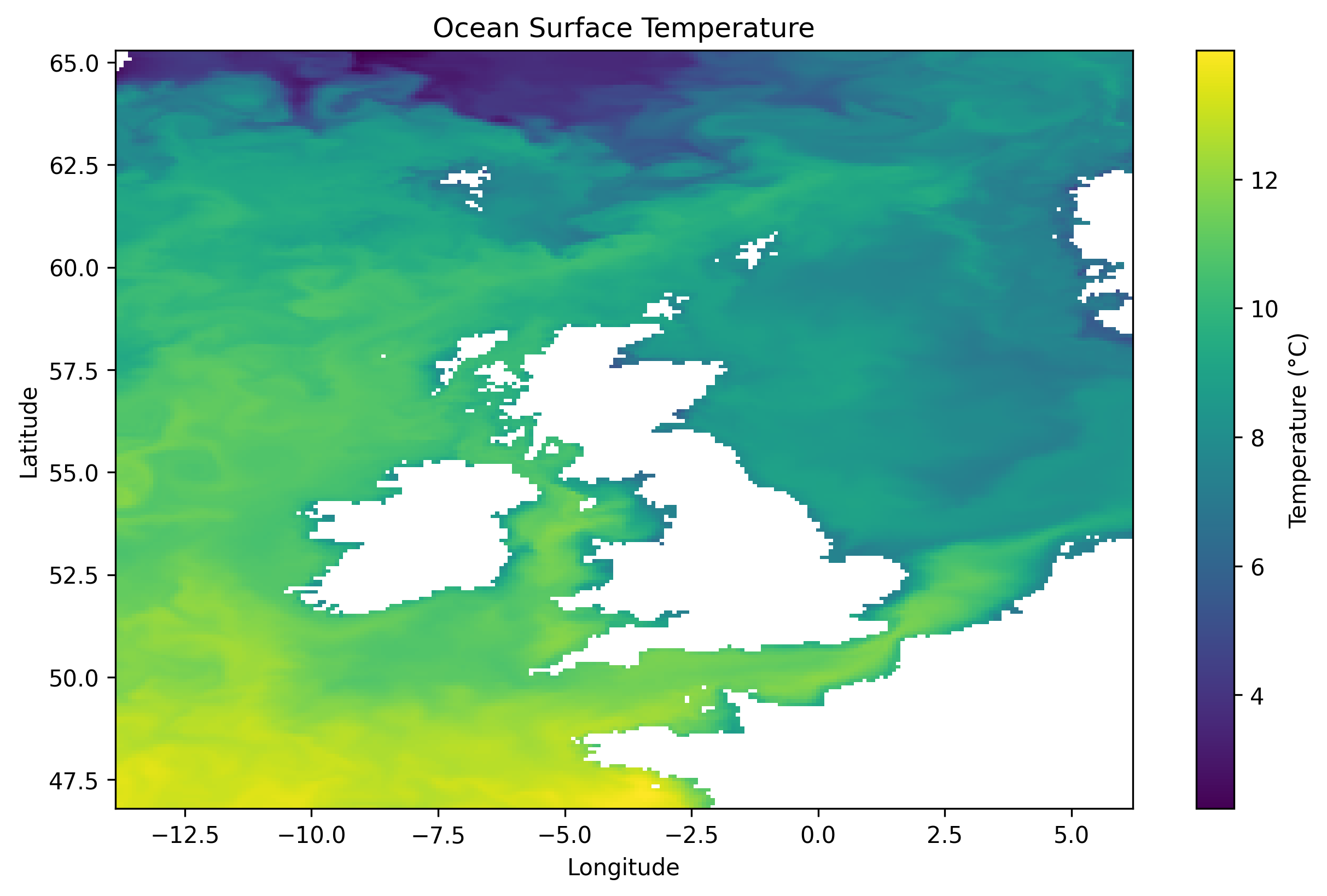
Visualizing a 2D temperature slice. The depth that will be targetted is the surface, e.g. 0.49m.
poetry run visualise_slice_static --data-file <netcdf_filename.nc>
The output produced will be a .png file, such as:
Visualise Slice - Interactive HTML file#
Visualizing a 2D temperature slice in an interactive HTML file, allowing for a time series to be visualised.
poetry run visualise_slice --target_depth 0 --animation_speed 100 --data-file <netcdf_filename.nc>
The command above will create an interactive HTML file, that will have each timestep in the animation last for 100 milliseconds (--animation_speed) at the nearest depth to the closest depth (--target_depth), in this case 0.49m. For the above command the output produced will be:
When run within your own space the file produced will be output/original_temperature_2d_interactive.html.
Visualise Cube - Interactive HTML file#
Visualizing a 3D temperature slice in an interactive HTML file, allowing for a time series to be visualised.
poetry run visualise_cube --num_depths 5 --num_time_steps 3 --data-file <netcdf_filename.nc>
The command above will create an interactive HTML file, that will visualise the first 5 depths, for 3 time steps. For the above command the output produced will be:
When run within your own space the file produced will be `output/original_temperature_3d_interactive.html`.Summarising Data#
Calculates and prints summary statistics for temperature data in a specified NetCDF file. Prints its mean, max, min, and standard deviation. Also provides information about the dataset’s dimensions and coordinates.
poetry run summary
The above command will print out the summary of the data on the original datafile downloaded from Copernicus. The above command will output the following:
The dimensions of the data is: (5, 50, 222, 241)
Temperature Summary Statistics:
Mean temperature: 8.56154727935791
Max temperature: 14.050389289855957
Min temperature: -2.591400146484375
Standard deviation: 3.1273183822631836

Dataset Dimensions and Coordinates:
<xarray.Dataset>
Dimensions:    (depth: 50, latitude: 222, longitude: 241, time: 5)
Coordinates:
  * depth      (depth) float32 0.494 1.541 2.646 ... 5.275e+03 5.728e+03
  * latitude   (latitude) float32 46.83 46.92 47.0 47.08 ... 65.08 65.17 65.25
  * longitude  (longitude) float32 -13.83 -13.75 -13.67 ... 6.0 6.083 6.167
  * time       (time) datetime64[ns] 2024-01-01 ... 2024-01-02
Data variables:
    thetao     (time, depth, latitude, longitude) float32 13.47 13.42 ... nan
Attributes: (12/14)
    Conventions:                   CF-1.6
    area:                          GLOBAL
    contact:                       servicedesk.cmems@mercator-ocean.eu
    credit:                        E.U. Copernicus Marine Service Information...
    institution:                   Mercator Ocean
    licence:                       http://marine.copernicus.eu/services-portf...
    ...                            ...
    product_user_manual:           http://marine.copernicus.eu/documents/PUM/...
    quality_information_document:  http://marine.copernicus.eu/documents/QUID...
    references:                    http://marine.copernicus.eu
    source:                        MERCATOR GLO12
    title:                         Instantaneous fields for product GLOBAL_AN...
    copernicusmarine_version:      1.3.4
Bringing It All Together#
The goal of this is to bring together what has been discussed so far in this course. You are provided with two options for what you want to tackle in this section; you could:
Develop a NumPy and CuPy version of the temperature diffusion model created.
Profile the NumPy and CuPy code provided with the tools discussed so far and understand where computation time is being spent and provide associated plots and a report on the performance of the different solutions to the problem.
Pseudocode#
The psuedocode that implements the diffusion loop is:
1. For each timestep from 1 to num_timesteps:
   2. Copy the current temperature values to a temporary array (temp_copy)
   3. Initialize arrays for neighbor sums and neighbor counts with zeros
   4. For each valid cell (ignoring boundaries):
      5. Calculate the sum of neighboring cells:
         - Add the value of the front neighbor if valid
         - Add the value of the back neighbor if valid
         - Add the value of the left neighbor if valid
         - Add the value of the right neighbor if valid
         - Add the value of the top neighbor if valid
         - Add the value of the bottom neighbor if valid
      6. Count the number of valid neighbors for each direction
   7. Update the cell's temperature:
      - New temperature = current temperature + diffusion coefficient * (neighbor_sum - 6 * current temperature) / neighbor_count
   8. Ensure invalid points (NaN) remain unchanged
   9. Update the main temperature array with the new values
The naive implementation of this problem is implemented within the function temperature_diffusion_purepython() in the file content/temperature_diffusion.py. A complete solution including reading and writing of .nc files is:
import xarray as xr
from pathlib import Path
import argparse
import time
import xarray as xr
import numpy as np
import cupy as cp
from tqdm import tqdm
import math
import copy


# Define the root directory
ROOT_DIR = Path(__file__).resolve().parent.parent
DATA_DIR = ROOT_DIR / "model_data"
DATA_FILE = "cmems_mod_glo_phy-thetao_anfc_0.083deg_PT6H-i_thetao_13.83W-6.17E_46.83N-65.25N_0.49-5727.92m_2024-01-01-2024-01-01.nc"

OUTPUT_FILE_NUMPY = "predicted_temperatures_numpy.nc"
OUTPUT_FILE_CUPY = "predicted_temperatures_cupy.nc"
OUTPUT_FILE_PUREPYTHON = "predicted_temperatures_purepython.nc"


# Load the NetCDF data
def load_data():
    file_path = DATA_DIR / DATA_FILE
    return xr.open_dataset(file_path)


def save_to_netcdf(data, new_temperature, output_file_path, num_timesteps):
    # Adjust new_temperature to have only num_timesteps or fewer
    new_temperature = new_temperature[:num_timesteps]  # Only include the desired number of timesteps

    # Generate a new time coordinate as a sequence of numbers (1, 2, ..., num_timesteps)
    time_coord = range(1, num_timesteps + 1)

    # Create a new dataset with original depth, latitude, and longitude coordinates
    output_data = xr.Dataset(
        {'thetao': (('time', 'depth', 'latitude', 'longitude'), new_temperature)},
        coords={
            'time': time_coord,  # Sequential time coordinate
            'depth': data['depth'].values,  # Use original depth coordinates
            'latitude': data['latitude'].values,  # Use original latitude coordinates
            'longitude': data['longitude'].values  # Use original longitude coordinates
        },
    )
    output_data.to_netcdf(output_file_path, engine='netcdf4')

def temperature_diffusion_purepython(data, num_timesteps, diffusion_coeff=0.1):
    # Pull raw array and get dims
    raw = data['thetao'].values              # shape (time, depth, lat, lon)
    depth, lat, lon = raw.shape[1], raw.shape[2], raw.shape[3]

    # Initial snapshot at t=0, as Python lists
    initial = raw[0]                         # shape (depth, lat, lon)
    temperature = []
    for _ in range(num_timesteps):
        # deep copy initial for each timestep
        plane = []
        for d in range(depth):
            plane.append([ [ float(initial[d][i][j]) for j in range(lon) ]
                           for i in range(lat) ])
        temperature.append(plane)

    # Summary stats (very slow!)
    flat = []
    for t in range(num_timesteps):
        for d in range(depth):
            for i in range(lat):
                for j in range(lon):
                    v = temperature[t][d][i][j]
                    if not math.isnan(v):
                        flat.append(v)
    flat_sorted = sorted(flat)

    # Precompute mask of valid ocean points
    mask = [[[ [ not math.isnan(temperature[t][d][i][j])
                 for j in range(lon) ]
               for i in range(lat) ]
             for d in range(depth) ]
           for t in range(num_timesteps)]

    # Prepare output buffer
    new_temperature = copy.deepcopy(temperature)
    timestep_durations = []

    # Diffusion loop
    for t in range(num_timesteps):
        start = time.time()
        for d in range(1, depth-1):
            for i in range(1, lat-1):
                for j in range(1, lon-1):
                    if mask[t][d][i][j]:
                        center = temperature[t][d][i][j]
                        total = 0.0
                        count = 0
                        # 6 neighbors
                        for dd, ii, jj in (
                            (d-1,i,j), (d+1,i,j),
                            (d,i-1,j), (d,i+1,j),
                            (d,i,j-1), (d,i,j+1)
                        ):
                            if mask[t][dd][ii][jj]:
                                total += temperature[t][dd][ii][jj]
                                count += 1
                        # apply diffusion
                        if count > 0:
                            delta = diffusion_coeff * (total - count*center) / count
                        else:
                            delta = 0.0
                        new_temperature[t][d][i][j] = center + delta
        timestep_durations.append(time.time() - start)
        # copy new → temperature for next step
        temperature[t] = copy.deepcopy(new_temperature[t])

    final = _np.array(new_temperature)

    # Save result
    save_to_netcdf(data, final, DATA_DIR / OUTPUT_FILE_PUREPYTHON, num_timesteps)

    total = sum(timestep_durations)
    avg = total / num_timesteps

    print(f"PurePython model completed in {total:.4f} seconds. "
          f"Average time per timestep: {avg:.4f} seconds.")

def run_diffusion_purepython():
    parser = argparse.ArgumentParser(description="Run 3D Diffusion Model in pure Python")
    parser.add_argument("--num_timesteps", type=int, default=300, help="Number of Timesteps")
    args = parser.parse_args()
    temperature_diffusion_purepython(data=load_data(), num_timesteps=args.num_timesteps)


if __name__ == "__main__":
    run_diffusion_purepython()
Example Results#
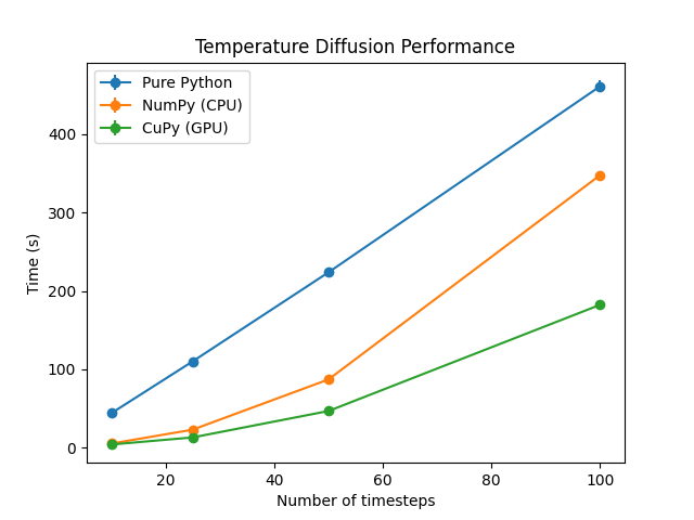
GPU Name |
CPU Name |
Method |
Time Steps |
Mean Time (s) |
Std Dev (s) |
|---|---|---|---|---|---|
NVIDIA H100 NVL |
AMD EPYC 9V84 96-Core Processor |
Pure Python |
10 |
43.698821 |
0.08423 |
NVIDIA H100 NVL |
AMD EPYC 9V84 96-Core Processor |
Pure Python |
25 |
110.014916 |
0.939186 |
NVIDIA H100 NVL |
AMD EPYC 9V84 96-Core Processor |
Pure Python |
50 |
223.748059 |
1.287061 |
NVIDIA H100 NVL |
AMD EPYC 9V84 96-Core Processor |
Pure Python |
100 |
461.348654 |
7.234776 |
NVIDIA H100 NVL |
AMD EPYC 9V84 96-Core Processor |
NumPy (CPU) |
10 |
4.980454 |
0.173302 |
NVIDIA H100 NVL |
AMD EPYC 9V84 96-Core Processor |
NumPy (CPU) |
25 |
22.786639 |
0.205813 |
NVIDIA H100 NVL |
AMD EPYC 9V84 96-Core Processor |
NumPy (CPU) |
50 |
86.931572 |
0.502695 |
NVIDIA H100 NVL |
AMD EPYC 9V84 96-Core Processor |
NumPy (CPU) |
100 |
347.883550 |
3.980833 |
NVIDIA H100 NVL |
AMD EPYC 9V84 96-Core Processor |
CuPy (GPU) |
10 |
3.854066 |
0.140653 |
NVIDIA H100 NVL |
AMD EPYC 9V84 96-Core Processor |
CuPy (GPU) |
25 |
12.885241 |
0.022276 |
NVIDIA H100 NVL |
AMD EPYC 9V84 96-Core Processor |
CuPy (GPU) |
50 |
46.622783 |
0.178398 |
NVIDIA H100 NVL |
AMD EPYC 9V84 96-Core Processor |
CuPy (GPU) |
100 |
182.261322 |
0.193946 |
Exercise: Approaching The Problem You Want#
Building on the “naive” pure-Python diffusion above, your task is to explore and extend the code in a way that resonates with you, some routes you could take include:
Implement Optimized Variants
Rewrite the naive nested-loop Python implementation using NumPy vectorized operations to leverage contiguous array arithmetic.
Translate your NumPy version to CuPy so that the heavy array work runs on the GPU.
Performance Profiling & Scaling
Use Python’s
time,cProfile,NVIDIA NSightor some other tool to measure per-timestep costs for each implementation (naive, NumPy, CuPy).Generate scaling plots to quantify speedup factors and identify bottlenecks.
Memory Footprint & Out-of-Core Strategies
Experiment with different depth/latitude/longitude resolutions and observe GPU vs. CPU memory usage.
If you exhaust GPU memory, explore chunking or out-of-core techniques (e.g. processing one depth-slice at a time).
Domain Decomposition & Halo Exchanges
Split the 3D grid into sub-domains (e.g. along latitude/longitude) for parallel processing.
Implement halo (ghost) cell exchanges between sub-domains to maintain correctness at boundaries when updating temperature.
Multi-GPU Offloading
Use CuPy’s multi-GPU capabilities (for example,
cupy.cuda.Device) to assign different sub-domains to separate GPUs.
Advanced Kernel Optimizations
Investigate writing custom CUDA kernels (via CuPy RawKernels) or use Numba JIT to fuse loops and reduce launch overhead.
Profile memory access patterns; consider tiling or pitched memory layouts to improve cache efficiency.
Visualization & Validation
Create interactive Plotly or static Matplotlib visuals of both the diffusion results and your profiling data.
Verify that all implementations produce numerically consistent outputs (e.g., compare final temperature fields).
Feel free to pick one or more of these directions or combine them—to deepen your understanding of high-performance computing with Python, NumPy, and CuPy. Note that not all of the topics above we have tackled in this course, so you may need to do some independent research if you choose some of the advanced topics. Good luck!