

Connected Component Analysis#
Questions
How to extract separate objects from an image and describe these objects quantitatively.
Objectives
Understand the term object in the context of images.
Learn about pixel connectivity.
Learn how Connected Component Analysis (CCA) works.
Use CCA to produce an image that highlights every object in a different colour.
Characterise each object with numbers that describe its appearance.
Objects#
In the Thresholding episode we have covered dividing an image into foreground and background pixels. In the shapes example image, we considered the coloured shapes as foreground objects on a white background.
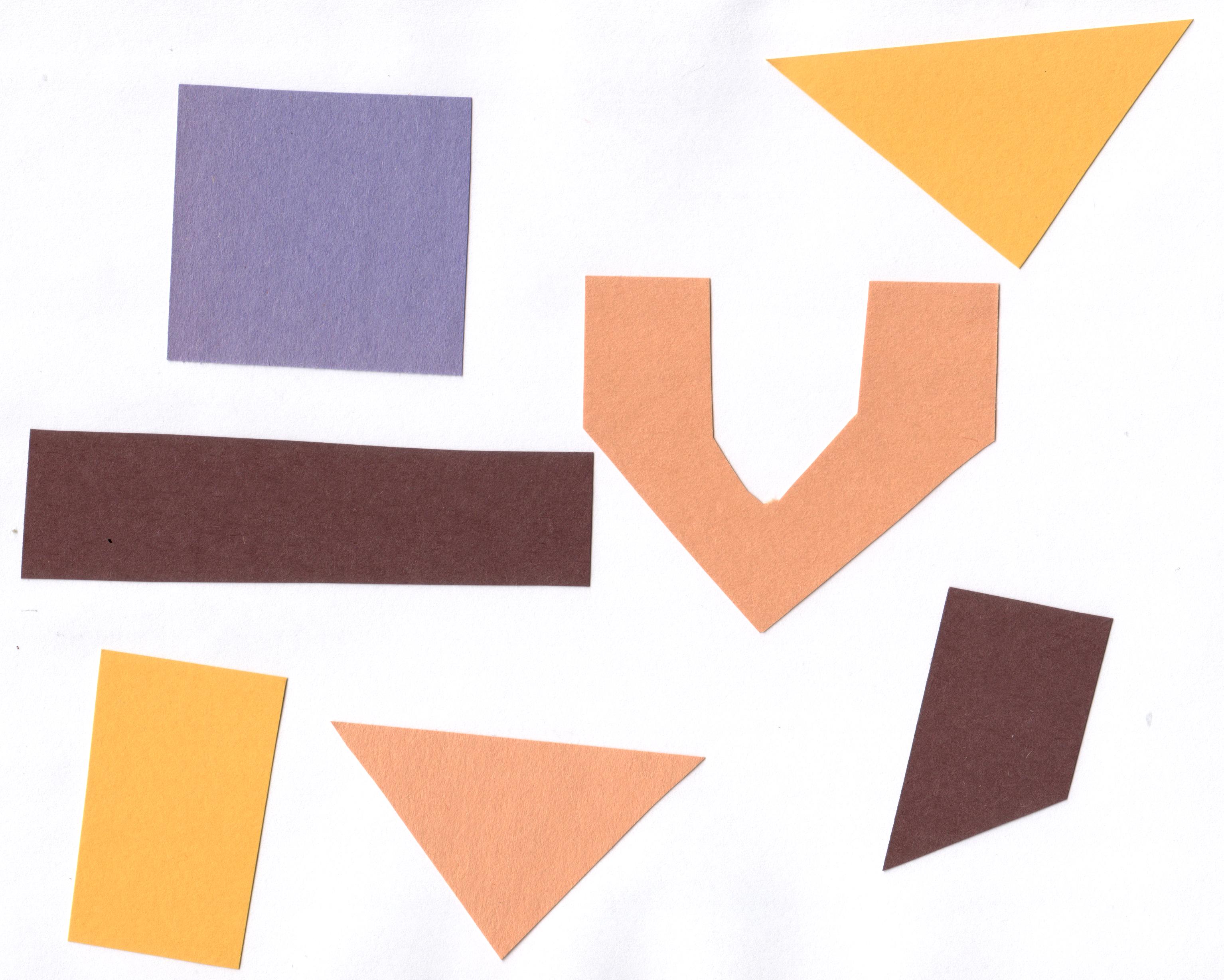
In thresholding we went from the original image to this version:
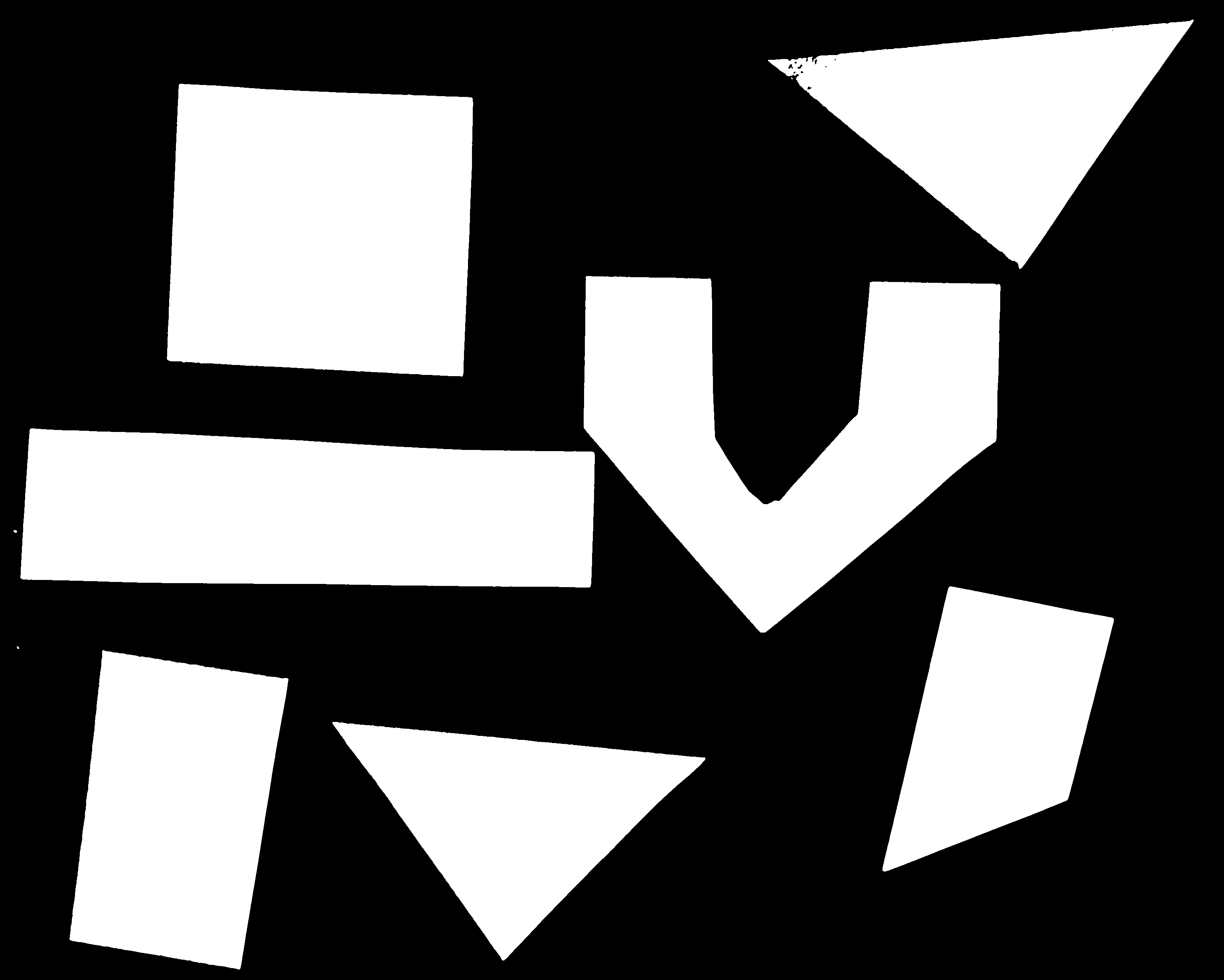
Here, we created a mask that only highlights the parts of the image
that we find interesting, the objects.
All objects have pixel value of True while the background pixels are False.
By looking at the mask image, one can count the objects that are present in the image (7). But how did we actually do that, how did we decide which lump of pixels constitutes a single object?
Pixel Neighborhoods#
In order to decide which pixels belong to the same object, one can exploit their neighborhood: pixels that are directly next to each other and belong to the foreground class can be considered to belong to the same object.
Let’s discuss the concept of pixel neighborhoods in more detail.
Consider the following mask “image” with 8 rows, and 8 columns.
For the purpose of illustration, the digit 0 is used to represent
background pixels, and the letter X is used to represent
object pixels (foreground).
0 0 0 0 0 0 0 0
0 X X 0 0 0 0 0
0 X X 0 0 0 0 0
0 0 0 X X X 0 0
0 0 0 X X X X 0
0 0 0 0 0 0 0 0
The pixels are organised in a rectangular grid.
In order to understand pixel neighborhoods
we will introduce the concept of “jumps” between pixels.
The jumps follow two rules:
First rule is that one jump is only allowed along the column, or the row.
Diagonal jumps are not allowed.
So, from a centre pixel, denoted with o,
only the pixels indicated with a 1 are reachable:
- 1 -
1 o 1
- 1 -
The pixels on the diagonal (from o) are not reachable with a single jump,
which is denoted by the -.
The pixels reachable with a single jump form the 1-jump neighborhood.
The second rule states that in a sequence of jumps,
one may only jump in row and column direction once -> they have to be orthogonal.
An example of a sequence of orthogonal jumps is shown below.
Starting from o the first jump goes along the row to the right.
The second jump then goes along the column direction up.
After this,
the sequence cannot be continued as a jump has already been made
in both row and column direction.
- - 2
- o 1
- - -
All pixels reachable with one, or two jumps form the 2-jump neighborhood.
The grid below illustrates the pixels reachable from
the centre pixel o with a single jump, highlighted with a 1,
and the pixels reachable with 2 jumps with a 2.
2 1 2
1 o 1
2 1 2
We want to revisit our example image mask from above and apply
the two different neighborhood rules.
With a single jump connectivity for each pixel, we get two resulting objects,
highlighted in the image with A’s and B’s.
0 0 0 0 0 0 0 0
0 A A 0 0 0 0 0
0 A A 0 0 0 0 0
0 0 0 B B B 0 0
0 0 0 B B B B 0
0 0 0 0 0 0 0 0
In the 1-jump version,
only pixels that have direct neighbors along rows or columns are considered connected.
Diagonal connections are not included in the 1-jump neighborhood.
With two jumps, however, we only get a single object A because pixels are also
considered connected along the diagonals.
0 0 0 0 0 0 0 0
0 A A 0 0 0 0 0
0 A A 0 0 0 0 0
0 0 0 A A A 0 0
0 0 0 A A A A 0
0 0 0 0 0 0 0 0
Exercise: Object counting (optional, not included in timing)#
How many objects with 1 orthogonal jump, how many with 2 orthogonal jumps?
0 0 0 0 0 0 0 0
0 X 0 0 0 X X 0
0 0 X 0 0 0 0 0
0 X 0 X X X 0 0
0 X 0 X X 0 0 0
0 0 0 0 0 0 0 0
1 jump:
a) 1 b) 5 c) 2
2 jumps:
a) 2 b) 3 c) 5
Solution
1 jump - b) 5
2 jump - a) 2
Jumps and neighborhoods
We have just introduced how you can reach different neighboring pixels by performing one or more orthogonal jumps. We have used the terms 1-jump and 2-jump neighborhood. There is also a different way of referring to these neighborhoods: the 4- and 8-neighborhood. With a single jump you can reach four pixels from a given starting pixel. Hence, the 1-jump neighborhood corresponds to the 4-neighborhood. When two orthogonal jumps are allowed, eight pixels can be reached, so the 2-jump neighborhood corresponds to the 8-neighborhood.
Connected Component Analysis#
In order to find the objects in an image, we want to employ an
operation that is called Connected Component Analysis (CCA).
This operation takes a binary image as an input.
Usually, the False value in this image is associated with background pixels,
and the True value indicates foreground, or object pixels.
Such an image can be produced, e.g., with thresholding.
Given a thresholded image,
the connected component analysis produces a new labeled image with integer pixel values.
Pixels with the same value, belong to the same object.
scikit-image provides connected component analysis in the function ski.measure.label().
Let us add this function to the already familiar steps of thresholding an image.
First, import the packages needed for this episode:
import imageio.v3 as iio
import ipympl
import matplotlib.pyplot as plt
import numpy as np
import skimage as ski

%matplotlib widget
In this episode, we will use the ski.measure.label function to perform the CCA.
Next, we define a reusable Python function connected_components:
def connected_components(filename, sigma=1.0, t=0.5, connectivity=2):
    # load the image
    image = iio.imread(filename)
    # convert the image to grayscale
    gray_image = ski.color.rgb2gray(image)
    # denoise the image with a Gaussian filter
    blurred_image = ski.filters.gaussian(gray_image, sigma=sigma)
    # mask the image according to threshold
    binary_mask = blurred_image < t
    # perform connected component analysis
    labeled_image, count = ski.measure.label(binary_mask,
                                             connectivity=connectivity, return_num=True)
    return labeled_image, count
The first four lines of code are familiar from the Thresholding episode.
Then we call the ski.measure.label function.
This function has one positional argument where we pass the binary_mask,
i.e., the binary image to work on.
With the optional argument connectivity,
we specify the neighborhood in units of orthogonal jumps.
For example,
by setting connectivity=2 we will consider the 2-jump neighborhood introduced above.
The function returns a labeled_image where each pixel has
a unique value corresponding to the object it belongs to.
In addition, we pass the optional parameter return_num=True to return
the maximum label index as count.
Optional parameters and return values
The optional parameter return_num changes the data type that is
returned by the function ski.measure.label.
The number of labels is only returned if return_num is True.
Otherwise, the function only returns the labeled image.
This means that we have to pay attention when assigning
the return value to a variable.
If we omit the optional parameter return_num or pass return_num=False,
we can call the function as
labeled_image = ski.measure.label(binary_mask)
If we pass return_num=True, the function returns a tuple and we
can assign it as
labeled_image, count = ski.measure.label(binary_mask, return_num=True)
If we used the same assignment as in the first case,
the variable labeled_image would become a tuple,
in which labeled_image[0] is the image
and labeled_image[1] is the number of labels.
This could cause confusion if we assume that labeled_image
only contains the image and pass it to other functions.
If you get an
AttributeError: 'tuple' object has no attribute 'shape'
or similar, check if you have assigned the return values consistently
with the optional parameters.
We can call the above function connected_components and
display the labeled image like so:
labeled_image, count = connected_components(filename="data/shapes-01.jpg", sigma=2.0, t=0.9, connectivity=2)

fig, ax = plt.subplots()
ax.imshow(labeled_image)
ax.set_axis_off();
Do you see an empty image?
If you are using an older version of Matplotlib you might get a warning
UserWarning: Low image data range; displaying image with stretched contrast.
or just see a visually empty image.
What went wrong?
When you hover over the image,
the pixel values are shown as numbers in the lower corner of the viewer.
You can see that some pixels have values different from 0,
so they are not actually all the same value.
Let’s find out more by examining labeled_image.
Properties that might be interesting in this context are dtype,
the minimum and maximum value.
We can print them with the following lines:
print("dtype:", labeled_image.dtype)
print("min:", np.min(labeled_image))
print("max:", np.max(labeled_image))
Examining the output can give us a clue why the image appears empty.
dtype: int32
min: 0
max: 11
The dtype of labeled_image is int32.
This means that values in this image range from -2 ** 31 to 2 ** 31 - 1.
Those are really big numbers.
From this available space we only use the range from 0 to 11.
When showing this image in the viewer,
it may squeeze the complete range into 256 gray values.
Therefore, the range of our numbers does not produce any visible variation. One way to rectify this
is to explicitly specify the data range we want the colormap to cover:
fig, ax = plt.subplots()
ax.imshow(labeled_image, vmin=np.min(labeled_image), vmax=np.max(labeled_image))
Note this is the default behaviour for newer versions of matplotlib.pyplot.imshow.
Alternatively we could convert the image to RGB and then display it.
Suppressing outputs in Jupyter Notebooks
We just used ax.set_axis_off(); to hide the axis from the image for a visually cleaner figure. The
semicolon is added to suppress the output(s) of the statement, in this case
the axis limits. This is specific to Jupyter Notebooks.
We can use the function ski.color.label2rgb()
to convert the 32-bit grayscale labeled image to standard RGB colour
(recall that we already used the ski.color.rgb2gray() function
to convert to grayscale).
With ski.color.label2rgb(),
all objects are coloured according to a list of colours that can be customised.
We can use the following commands to convert and show the image:
# convert the label image to color image
colored_label_image = ski.color.label2rgb(labeled_image, bg_label=0)

fig, ax = plt.subplots()
ax.imshow(colored_label_image)
ax.set_axis_off();
Exercise: How many objects are in that image (15 min)#
Now, it is your turn to practice.
Using the function connected_components,
find two ways of printing out the number of objects found in the image.
What number of objects would you expect to get?
How does changing the sigma and threshold values influence the result?
Solution
As you might have guessed, the return value count already
contains the number of objects found in the image. So it can simply be printed
with
print("Found", count, "objects in the image.")
But there is also a way to obtain the number of found objects from
the labeled image itself.
Recall that all pixels that belong to a single object
are assigned the same integer value.
The connected component algorithm produces consecutive numbers.
The background gets the value 0,
the first object gets the value 1,
the second object the value 2, and so on.
This means that by finding the object with the maximum value,
we also know how many objects there are in the image.
We can thus use the np.max function from NumPy to
find the maximum value that equals the number of found objects:
num_objects = np.max(labeled_image)
print("Found", num_objects, "objects in the image.")
Invoking the function with sigma=2.0, and threshold=0.9,
both methods will print
Found 11 objects in the image.
Lowering the threshold will result in fewer objects. The higher the threshold is set, the more objects are found. More and more background noise gets picked up as objects. Larger sigmas produce binary masks with less noise and hence a smaller number of objects. Setting sigma too high bears the danger of merging objects.
You might wonder why the connected component analysis with sigma=2.0,
and threshold=0.9 finds 11 objects, whereas we would expect only 7 objects.
Where are the four additional objects?
With a bit of detective work, we can spot some small objects in the image,
for example, near the left border.
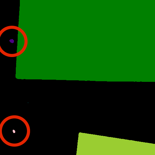
For us it is clear that these small spots are artifacts and
not objects we are interested in.
But how can we tell the computer?
One way to calibrate the algorithm is to adjust the parameters for
blurring (sigma) and thresholding (t),
but you may have noticed during the above exercise that
it is quite hard to find a combination that produces the right output number.
In some cases, background noise gets picked up as an object.
And with other parameters,
some of the foreground objects get broken up or disappear completely.
Therefore, we need other criteria to describe desired properties of the objects
that are found.
Morphometrics - Describe object features with numbers#
Morphometrics is concerned with the quantitative analysis of objects and
considers properties such as size and shape.
For the example of the images with the shapes,
our intuition tells us that the objects should be of a certain size or area.
So we could use a minimum area as a criterion for when an object should be detected.
To apply such a criterion,
we need a way to calculate the area of objects found by connected components.
Recall how we determined the root mass in
the Thresholding episode
by counting the pixels in the binary mask.
But here we want to calculate the area of several objects in the labeled image.
The scikit-image library provides the function ski.measure.regionprops
to measure the properties of labeled regions.
It returns a list of RegionProperties that describe each connected region in the images.
The properties can be accessed using the attributes of the RegionProperties data type.
Here we will use the properties "area" and "label".
You can explore the scikit-image documentation to learn about other properties available.
We can get a list of areas of the labeled objects as follows:
# compute object features and extract object areas
object_features = ski.measure.regionprops(labeled_image)
object_areas = [objf["area"] for objf in object_features]
object_areas
[318539.0,
 1.0,
 523207.0,
 496622.0,
 517330.0,
 143.0,
 256215.0,
 1.0,
 69.0,
 338787.0,
 265767.0]
Exercise: Plot a histogram of the object area distribution (10 min)#
Similar to how we determined a “good” threshold in the Thresholding episode, it is often helpful to inspect the histogram of an object property. For example, we want to look at the distribution of the object areas.
Create and examine a histogram of the object areas obtained with
ski.measure.regionprops.What does the histogram tell you about the objects?
Solution
The histogram can be plotted with
fig, ax = plt.subplots()
ax.hist(object_areas)
ax.set_xlabel("Area (pixels)")
ax.set_ylabel("Number of objects");
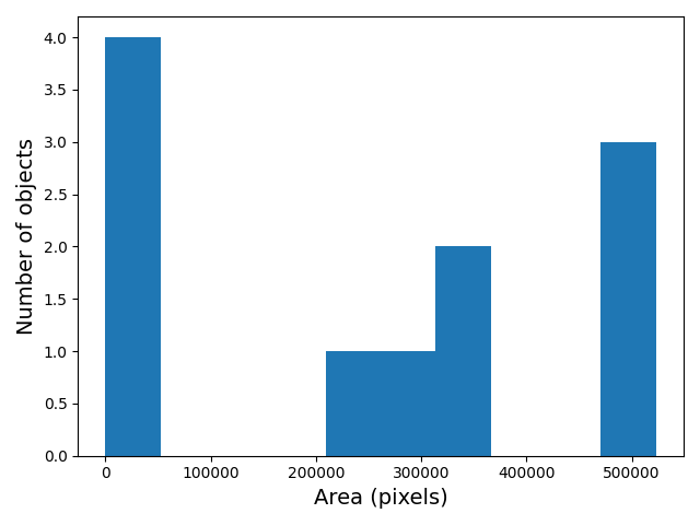
The histogram shows the number of objects (vertical axis) whose area is within a certain range (horizontal axis). The height of the bars in the histogram indicates the prevalence of objects with a certain area. The whole histogram tells us about the distribution of object sizes in the image. It is often possible to identify gaps between groups of bars (or peaks if we draw the histogram as a continuous curve) that tell us about certain groups in the image.
In this example, we can see that there are four small objects that
contain less than 50000 pixels.
Then there is a group of four (1+1+2) objects in
the range between 200000 and 400000,
and three objects with a size around 500000.
For our object count, we might want to disregard the small objects as artifacts,
i.e., we want to ignore the leftmost bar of the histogram.
We could use a threshold of 50000 as the minimum area to count.
In fact, the object_areas list already tells us that
there are fewer than 200 pixels in these objects.
Therefore, it is reasonable to require a minimum area of at least 200 pixels
for a detected object.
In practice, finding the “right” threshold can be tricky and
usually involves an educated guess based on domain knowledge.
Exercise: Filter objects by area (10 min)#
Now we would like to use a minimum area criterion to obtain a more accurate count of the objects in the image.
Find a way to calculate the number of objects by only counting objects above a certain area.
Solution
One way to count only objects above a certain area is to first create a list of those objects, and then take the length of that list as the object count. This can be done as follows:
min_area = 200
large_objects = []
for objf in object_features:
    if objf["area"] > min_area:
        large_objects.append(objf["label"])
print("Found", len(large_objects), "objects!")
Another option is to use NumPy arrays to create the list of large objects.
We first create an array object_areas containing the object areas,
and an array object_labels containing the object labels.
The labels of the objects are also returned by ski.measure.regionprops.
We have already seen that we can create boolean arrays using comparison operators.
Here we can use object_areas > min_area
to produce an array that has the same dimension as object_labels.
It can then be used to select the labels of objects whose area is
greater than min_area by indexing:
object_areas = np.array([objf["area"] for objf in object_features])
object_labels = np.array([objf["label"] for objf in object_features])
large_objects = object_labels[object_areas > min_area]
print("Found", len(large_objects), "objects!")
The advantage of using NumPy arrays is that
for loops and if statements in Python can be slow,
and in practice the first approach may not be feasible
if the image contains a large number of objects.
In that case, NumPy array functions turn out to be very useful because
they are much faster.
In this example, we can also use the np.count_nonzero function
that we have seen earlier together with the > operator to count
the objects whose area is above min_area.
n = np.count_nonzero(object_areas > min_area)
print("Found", n, "objects!")
For all three alternatives, the output is the same and gives the expected count of 7 objects.
Using functions from NumPy and other Python packages
Functions from Python packages such as NumPy are often more efficient and
require less code to write.
It is a good idea to browse the reference pages of numpy and skimage to
look for an available function that can solve a given task.
Exercise: Remove small objects (20 min)#
We might also want to exclude (mask) the small objects when plotting the labeled image.
Enhance the
connected_componentsfunction such that it automatically removes objects that are below a certain area that is passed to the function as an optional parameter.
Solution
To remove the small objects from the labeled image, we change the value of all pixels that belong to the small objects to the background label 0. One way to do this is to loop over all objects and set the pixels that match the label of the object to 0.
for object_id, objf in enumerate(object_features, start=1):
    if objf["area"] < min_area:
        labeled_image[labeled_image == objf["label"]] = 0
Here NumPy functions can also be used to eliminate
for loops and if statements.
Like above, we can create an array of the small object labels with
the comparison object_areas < min_area.
We can use another NumPy function, np.isin,
to set the pixels of all small objects to 0.
np.isin takes two arrays and returns a boolean array with values
True if the entry of the first array is found in the second array,
and False otherwise.
This array can then be used to index the labeled_image and
set the entries that belong to small objects to 0.
object_areas = np.array([objf["area"] for objf in object_features])
object_labels = np.array([objf["label"] for objf in object_features])
small_objects = object_labels[object_areas < min_area]
labeled_image[np.isin(labeled_image, small_objects)] = 0
An even more elegant way to remove small objects from the image is
to leverage the ski.morphology module.
It provides a function ski.morphology.remove_small_objects that
does exactly what we are looking for.
It can be applied to a binary image and
returns a mask in which all objects smaller than min_area are excluded,
i.e., their pixel values are set to False.
We can then apply ski.measure.label to the masked image:
object_mask = ski.morphology.remove_small_objects(binary_mask, min_size=min_area)
labeled_image, n = ski.measure.label(object_mask,
                                     connectivity=connectivity, return_num=True)
Using the scikit-image features, we can implement
the enhanced_connected_component as follows:
def enhanced_connected_components(filename, sigma=1.0, t=0.5, connectivity=2, min_area=0):
    image = iio.imread(filename)
    gray_image = ski.color.rgb2gray(image)
    blurred_image = ski.filters.gaussian(gray_image, sigma=sigma)
    binary_mask = blurred_image < t
    object_mask = ski.morphology.remove_small_objects(binary_mask, min_size=min_area)
    labeled_image, count = ski.measure.label(object_mask,
                                             connectivity=connectivity, return_num=True)
    return labeled_image, count
We can now call the function with a chosen min_area and
display the resulting labeled image:
labeled_image, count = enhanced_connected_components(filename="data/shapes-01.jpg", sigma=2.0, t=0.9,
                                                     connectivity=2, min_area=min_area)
colored_label_image = ski.color.label2rgb(labeled_image, bg_label=0)

fig, ax = plt.subplots()
ax.imshow(colored_label_image)
ax.set_axis_off();

print("Found", count, "objects in the image.")
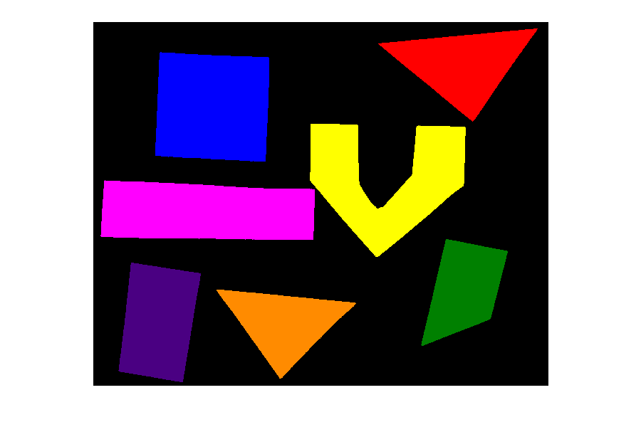
Found 7 objects in the image.
Note that the small objects are “gone” and we obtain the correct number of 7 objects in the image.
Exercise: Colour objects by area (optional, not included in timing)#
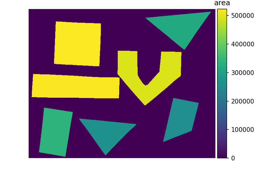
Finally, we would like to display the image with the objects coloured according to the magnitude of their area. In practice, this can be used with other properties to give visual cues of the object properties.
Solution
We already know how to get the areas of the objects from the regionprops.
We just need to insert a zero area value for the background
(to colour it like a zero size object).
The background is also labeled 0 in the labeled_image,
so we insert the zero area value in front of the first element of
object_areas with np.insert.
Then we can create a colored_area_image where we assign each pixel value
the area by indexing the object_areas with the label values in labeled_image.
object_areas = np.array([objf["area"] for objf in ski.measure.regionprops(labeled_image)])
# prepend zero to object_areas array for background pixels
object_areas = np.insert(0, obj=1, values=object_areas)
# create image where the pixels in each object are equal to that object's area
colored_area_image = object_areas[labeled_image]

fig, ax = plt.subplots()
im = ax.imshow(colored_area_image)
cbar = fig.colorbar(im, ax=ax, shrink=0.85)
cbar.ax.set_title("Area")
ax.set_axis_off();
Advanced indexing in NumPy
You may have noticed that in the solution, we have used the
labeled_image to index the array object_areas. This is an
example of advanced indexing in
NumPy.
The result is an array of the same shape as the labeled_image
whose pixel values are selected from object_areas according to
the object label. Hence the objects will be colored by area when
the result is displayed. Note that advanced indexing with an
integer array works slightly different than the indexing with a
Boolean array that we have used for masking. While Boolean array
indexing returns only the entries corresponding to the True
values of the index, integer array indexing returns an array
with the same shape as the index. You can read more about advanced
indexing in the NumPy
documentation.