

Multidimensional Data#
Questions
How can we use scikit-image to perform image processing tasks on multidimensional image data?
How can we visualise the results using Napari?
Objectives
Learn about multidimensional image data such as 3D volumetric stacks and timelapses.
Visualize multidimensional data interactively using Napari.
Learn to use the basic functionality of the Napari user interface including overlaying masks over images.
Construct an analysis workflow to measure the properties of 3D objects in a volumetric image stack.
In this episode we will move beyond 2D RGB image data and learn how to process and visualise multidimensional image data including 3D volumes and timelapse movies.
First, import the packages needed for this episode
import imageio.v3 as iio
import skimage as ski
import numpy as np
import napari
import matplotlib.pyplot as plt

%matplotlib widget
What is multidimensional image data?#
Image data is often more complex than individual 2D (xy) images and can have additional dimensionality and structure. Such multidimensional image data has many flavours including multichannel, 3D volumes and timelapse movies. It is possible to combine these flavours to produce higher n-dimensional data. For example a volumetric, multichannel, timelapse dataset would have a 5D (2+1+1+1) structure.
Multichannel image data#
In many applications we can have different 2D images, or channels, of the same spatial area. We have already seen a simple example of this in RGB colour images where we have 3 channels representing the red, green and blue components. Another example is in fluorescence microscopy where we could have images of different proteins. Modern techniques often allow for acquisition of more than 3 channels.
3D volumetric data#
Volumetric image data consists of an ordered sequence of 2D images (or slices) where each slice corresponds to a, typically evenly spaced, axial position. Such data is common in biomedical applications for example CT or MRI where it is used to reconstruct 3D volumes of organs such as the brain or heart.
Timelapse movies#
Timelapse movies are commonplace in everyday life. When you take a movie on your phone your acquire an ordered sequence of 2D images (or timepoints/frames) where each image corresponds to a specific point in time. Timelapse data is also common in scientific applications where we want to quantify changes over time. For example imaging the growth of cell cultures, bacterial colonies or plant roots over time.
Interactive image visualisation with Napari#
In the previous episodes we used matplotlib.pyplot.imshow() to display images. This is suitable
for basic visualisation of 2D multichannel image data but not well suited for more complex tasks
such as:
Interactive visualisation such as on-the-fly zooming in and out, rotation and toggling between channels.
Interactive image annotation. In the Drawing episode we used functions such as
ski.draw.rectangle()to programmatically annotate images but not in an interactive user-friendly way.Visualising 3D volumetric data either by toggling between slices or though a 3D rendering.
Visualising timelapse movies where the movie can be played and paused at specific timepoints.
Visualising complex higher order data (more than 3 dimensions) such as timelapse, volumetric multichannel images.
Napari is a Python library for
fast visualisation, annotation and analysis of n-dimensional image data. At its core is the
napari.Viewer class. Creating a
Viewer instance within a notebook will launch a Napari Graphical User Interface (GUI) with two-way
communication between the notebook and the GUI:
viewer = napari.Viewer()
The Napari Viewer displays data through
Layers. There are different Layer subclasses for
different types of data. Image Layers are for image data and Label Layers are for
masks/segmentations. There are also Layer subclasses for Points, Shapes, Surfaces etc. Let’s
load two RGB images and add them to the Viewer as Image Layers:
colonies_01 = iio.imread(uri="data/colonies-01.tif")
colonies_02 = iio.imread(uri="data/colonies-02.tif")
viewer.add_image(data=colonies_01, name="colonies_01", rgb=True)
viewer.add_image(data=colonies_02, name="colonies_02", rgb=True)
napari.utils.nbscreenshot(viewer)
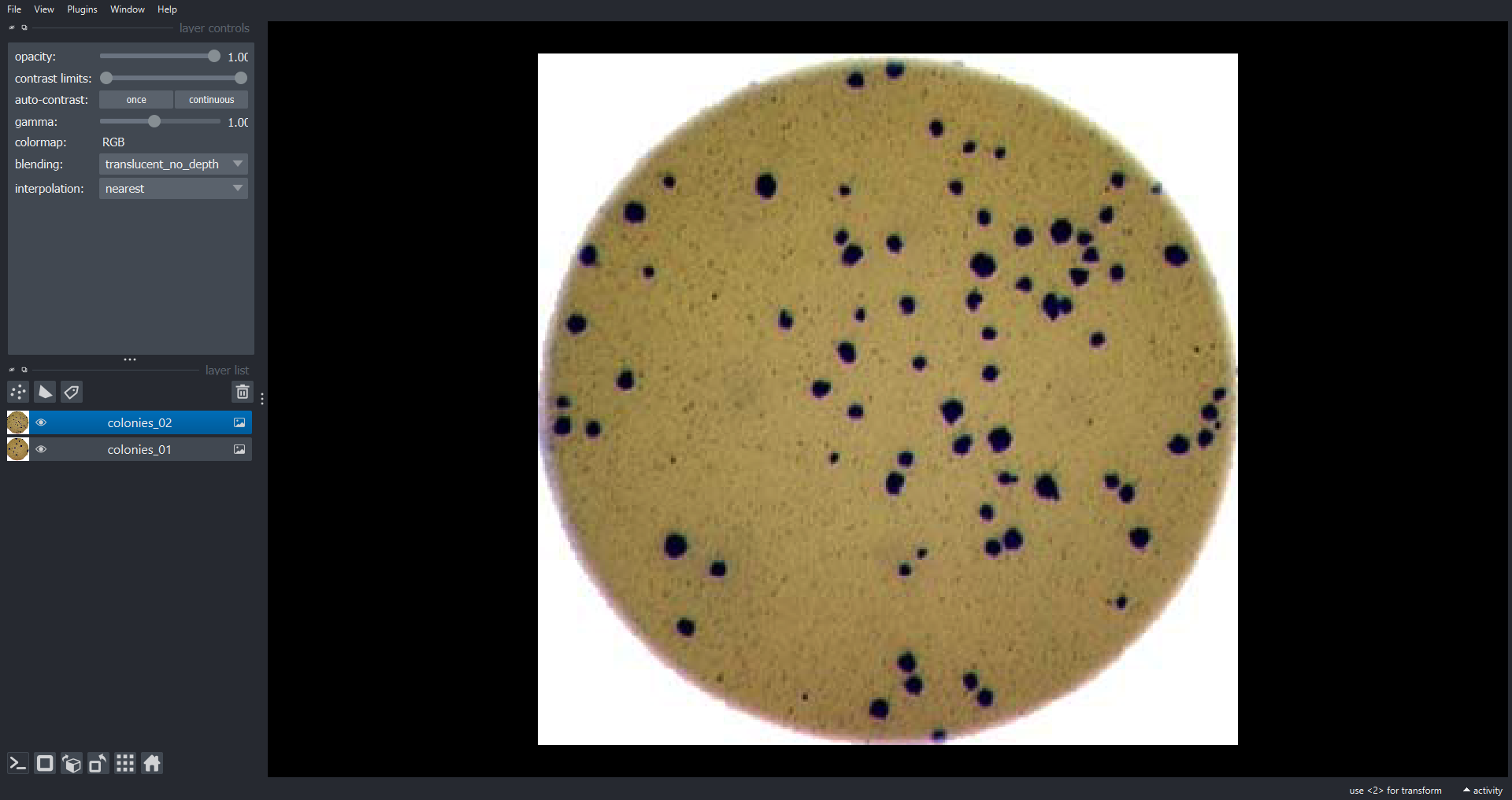
Here we use the viewer.add_image() function to add Image Layers to the Viewer. We set rgb=True
to display the three channel image as RGB. The napari.utils.nbscreenshot() function outputs a
screenshot of the Viewer to the notebook. Now lets look at some multichannel image data:
cells = iio.imread(uri="https://imagej.net/ij/images/FluorescentCells.jpg")
print(cells.shape)
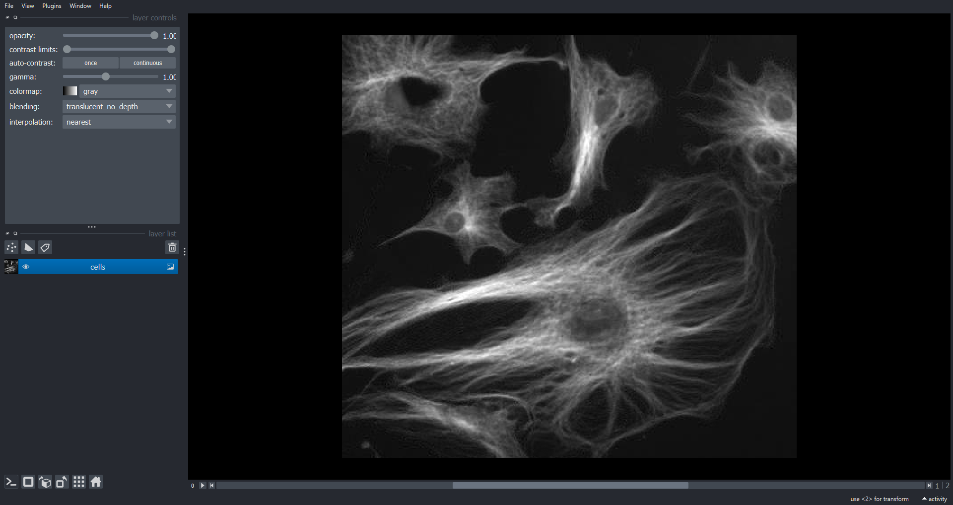
Like RGB data this image of cells also has three channels (stored in the first dimension of the
NumPy array). However, in this case we may want to visualise each channel independently. To do this
we do not set rgb=True when adding the Image Layer:
viewer.layers.clear()
viewer.add_image(data=cells, name="cells")
Clearing the Napari Viewer
When we want to close all Layers in a Viewer instance we can use viewer.layers.clear(). This
allows us to start fresh, alternatively we could close the existing Viewer and open a new one with
viewer = napari.Viewer(). We will use the first approach throughout this Episode but if any point
you accidentally close the Viewer you can just open a new one.
We can now scroll through the channels within Napari using the slider just below the image. This
approach will work with an arbitrary number of channels, not just three. With multichannel data it
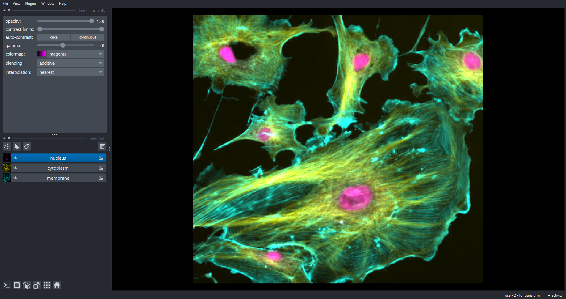
is common to visualise colour overlays of selected channels where each channel has a different
colour map. In Napari we can do this programmatically using the channel_axis variable:
viewer.layers.clear()
viewer.add_image(data=cells, name=["membrane", "cytoplasm", "nucleus"], channel_axis=2)
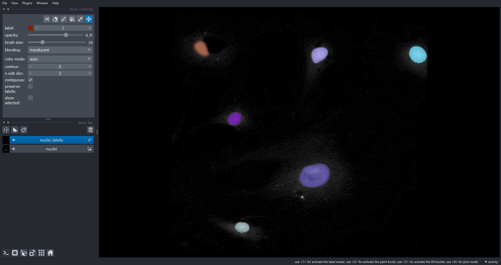
Using what we have learnt in the previous Episodes let’s segment the nuclei. First we produce a binary mask of the nuclei by blurring the nuclei channel image and thresholding with the Otsu approach. Subsequently, we label the connected components within the mask to identify individual nuclei:
blurred_nuclei = ski.filters.gaussian(cells[:, :, 2], sigma=2.0)
t = ski.filters.threshold_otsu(blurred_nuclei)
nuclei_mask = blurred_nuclei > t
nuclei_labels = ski.measure.label(nuclei_mask, connectivity=2, return_num=False)
Now lets display the nuclei channel and overlay the labels within Napari using a Label layer:
viewer.layers.clear()
viewer.add_image(data=cells[:, :, 2], name="nuclei")
viewer.add_labels(data=nuclei_labels, name="nuclei_labels")
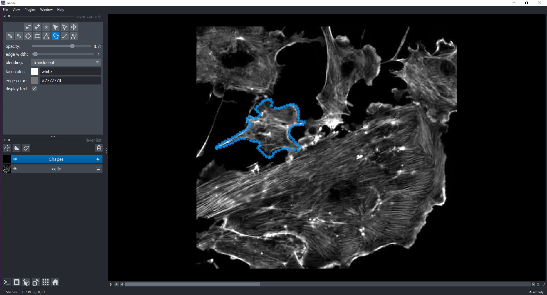
We can also interactively annotate images with shapes using a Shapes Layer. Let’s display all
three channels and then do this within the GUI:
viewer.layers.clear()
viewer.add_image(data=cells, name="cells")
# the instructor will demonstrate how to add a `Shapes` Layer and draw around cells using polygons
Exercise: Using Napari as an image viewer (20 min)#
In the Capstone challenge episode you made a function to count the number of
bacteria colonies in an image also producing a new image that highlights the colonies. Modify this
function to make use of Napari, as opposed to Matplotlib, to display both the original colony
image and the segmented individual colonies. Test this new function on "data/colonies-03.tif". If
you did not complete the Capstone challenge episode you can start with the function from the
solution there. Hints:
A
napari.Viewerobject should be passed to the function as an input parameter.The original image should be added to the Viewer as an
ImageLayer.The labelled colony image should be added to the Viewer as a
LabelLayer.
Solution
Your new function might look something like this:
def count_colonies_napari(image_filename, viewer, sigma=1.0, min_colony_size=10, connectivity=2):
    bacteria_image = iio.imread(image_filename)
    gray_bacteria = ski.color.rgb2gray(bacteria_image)
    blurred_image = ski.filters.gaussian(gray_bacteria, sigma=sigma)

    # create mask excluding the very bright pixels outside the dish
    # we dont want to include these when calculating the automated threshold
    mask = blurred_image < 0.90
    # calculate an automated threshold value within the dish using the Otsu method
    t = ski.filters.threshold_otsu(blurred_image[mask])
    # update mask to select pixels both within the dish and less than t
    mask = np.logical_and(mask, blurred_image < t)
    # remove objects smaller than specified area
    mask = ski.morphology.remove_small_objects(mask, min_size=min_colony_size)

    labeled_image, count = ski.measure.label(mask, return_num=True)
    print(f"There are {count} colonies in {image_filename}")

    # add the original image (RGB) to the Napari Viewer
    viewer.add_image(data=bacteria_image, name="bacteria", rgb=True)
    # add the labeled image to the Napari Viewer
    viewer.add_labels(data=labeled_image, name="colony masks")
To run this function on "data/colonies-03.tif":
viewer.layers.clear()  # or viewer = napari.Viewer() if you want a new Viewer
count_colonies_napari(image_filename="data/colonies-03.tif", viewer=viewer)
There are 260 colonies in data/colonies-03.tif

Exercise: Learning to use the Napari GUI (optional, not included in timing)#
Take some time to further familiarize yourself with the Napari GUI. You could load some of the course images and experiment with different features, or alternatively you could take a look at the official Viewer tutorial.
Napari plugins
Plugins extend Napari’s core functionality and allow you to add lots of cool and advanced features. There is an ever-increasing number of Napari plugins which are available from the Napari hub. For example:
napari-animation for making video annotations with key frames.
napari-segment-blobs-and-things-with-membranes for adding common image processing operations to the Tools menu.
napari-skimage-regionprops for measuring the properties of connected components from
LabelLayers.napari-pyclesperanto-assistant for GPU-accelerated image processing operations.
napari-clusters-plotter for clustering objects according to their properties including dimensionality reduction techniques like PCA and UMAP.
napari-acceleration-pixel-and-object-classification for Random Forest-based pixel and object classification.
cellpose-napari and stardist-napari for pretrained deep learning-based models to segment cells and nuclei.
napari-n2v for self-supervised deep learning-based denoising.
napari-assistant, a meta-plugin for building image processing workflows.
Getting help on image.sc
image.sc is a community forum for all software-oriented aspects of scientific imaging, particularly (but not limited to) image analysis, processing, acquisition, storage, and management. It’s a great place to get help and ask questions which are either general or specific to a particular tool. There are active sections for python, scikit-image and Napari.
Processing 3D volumetric data#
Recall that 3D volumetric data consists of an ordered sequence of images, or slices, each
corresponding to a specific axial position. As an example lets work with
skimage.data.cells3d() which is a 3D fluorescence microscopy image stack. From
the dataset documentation
we can see that the data has two channels (0: membrane, 1: nuclei). The dimensions are ordered
(z, channels, y, x) and each voxel has a size of (0.29 0.26 0.26) microns. A voxel is the 3D
equivalent of a pixel and the size specifies
the physical dimensions, in (z, y, x) order for this example. Note the size of the voxels in z
(axial) is larger than the voxel spacing in the xy dimensions (lateral). Let’s load the data and
visualise with Napari:
cells3d = ski.data.cells3d()
viewer.layers.clear()
viewer.add_image(data=cells3d, name=["membrane", "nucleus"], channel_axis=1)
print(cells3d.shape)
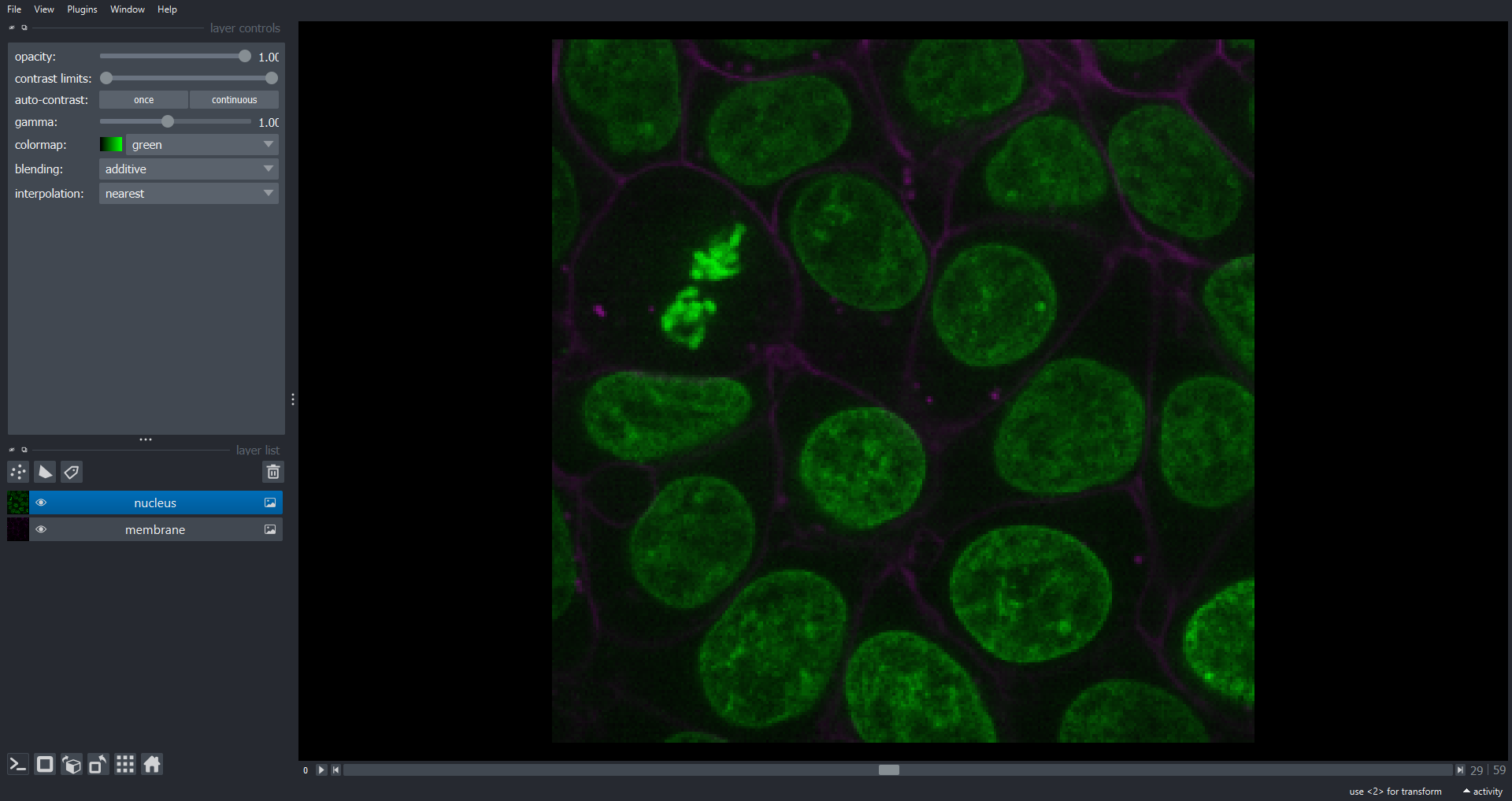
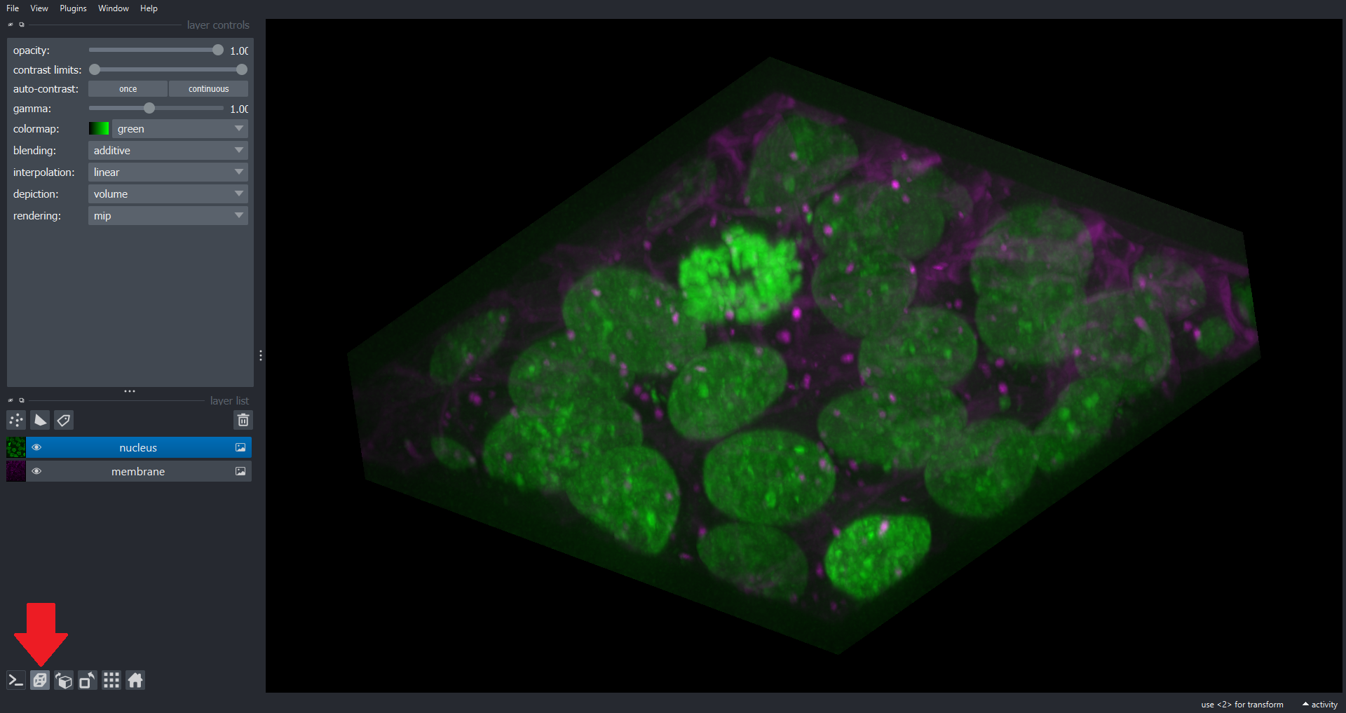
Note we now have a dimension slice to control which slice we are visualizing. You can also switch to a 3D rendering of the data:
Many of the scikit-image functions you have used throughout this Lesson work with 3D (or indeed nD)
image data. For example lets blur the nuclei channel using a 3D Gaussian filter and add the result
as a Image Layer to the Viewer:
# extract the nuclei channel
nuclei = cells3d[:, 1, :, :]
# store the voxel size as a NumPy array (in microns)
voxel_size = np.array([0.29, 0.26, 0.26])
# get sigma (std) values for each dimension that corresponds to 0.5 microns
sigma = 0.5 / voxel_size
# blur data with 3D Gaussian filter
blurred_nuclei = ski.filters.gaussian(nuclei, sigma=sigma)
# add to Napari Viewer
viewer.add_image(data=blurred_nuclei, name="nucleus_blurred")
print(sigma)
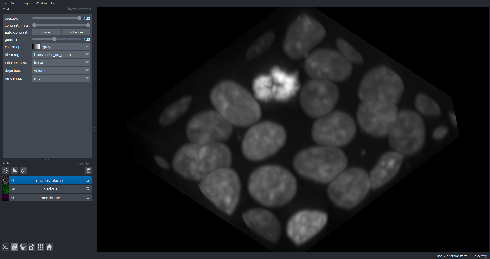
Note we have used a different sigma for the z dimension to allow for the different voxel dimensions, to produce a blur of 0.5 microns in each axis of real space.
Exercise: Segmenting objects in 3D (25 min)#
Write a workflow which:
Segments the nuclei within
skimage.data.cells3d()to produce a 3D labelled volume.Add the 3D labelled volume to a Napari Viewer as a
LabelLayer.Calculate the mean volume in microns^3 of all distinct objects (connected components) in your 3D labelled volume.
You will need to recall concepts from the Thresholding and the Connected Components Analysis episodes. Hints:
The 3D blurred nuclei volume we have just calculated makes a good starting point.
ski.morphology.remove_small_objects()is useful for removing small objects in masks. In 3D themin_sizeparameter specifies the minimum number of voxels a connected component should contain.In 3D we typically use
connectivity=3(as opposed toconnectivity=2for 2D data).ski.measure.regionprops()can be used to calculate the properties of connected components in 3D. The returned"area"property gives the volume of each object in voxels.
Solution
Starting with the 3D blurred nuclei volume as our starting point here is one potential solution that will segment the nuclei and add to the existing Napari Viewer:
# use an automated Otsu threshold to produce a binary mask of the nuclei
t = ski.filters.threshold_otsu(blurred_nuclei)
nuclei_mask = blurred_nuclei > t
# remove objects from the mask smaller than 5 microns^3
# np.prod(voxel_size) returns the volume of a voxel in microns^3
min_size = 5 / np.prod(voxel_size)
nuclei_mask = ski.morphology.remove_small_objects(nuclei_mask, min_size=min_size, connectivity=3)
# label 3D connected components
# we specify connectivity=3 but this is the default behaviour for 3D data
nuclei_labels = ski.measure.label(nuclei_mask, connectivity=3, return_num=False)
# add to Napari Viewer
viewer.add_labels(data=nuclei_labels, name="nuclei_labels")
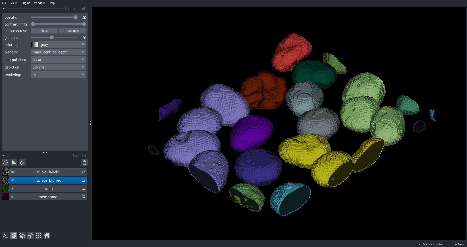
To extract the properties of the connected components we can use ski.measure.regionprops():
props = ski.measure.regionprops(nuclei_labels)
# get the cell volumes in pixels as a NumPy array
cell_volumes_voxels = np.array([objf["area"] for objf in props])
# get the mean and convert to microns^3
cell_volumes_mean = np.mean(cell_volumes_voxels) * np.prod(voxel_size)
f"There are {len(cell_volumes_voxels)} distinct objects with a mean volume of {cell_volumes_mean} microns^3"
‘There are 18 distinct objects with a mean volume of 784.6577237777778 microns^3’
Exercise: Intensity morphometrics (optional, not included in timing)#
It is common to want to retrieve properties of connected components which use the pixel intensities
from the original data. For example the mean, max, min or sum pixel intensity within each object.
Modify your solution from the previous exercise to also retrieve the mean intensity of the original
nuclei channel within each connected component. You may need to refer to
the ski.measure.regionprops() documentation.
Solution
props = ski.measure.regionprops(nuclei_labels, intensity_image=nuclei)
# get the cell volumes in pixels as a NumPy array
cell_volumes_pixels = np.array([objf["area"] for objf in props])
# get the mean and convert to microns^3
cell_volumes_mean = np.mean(cell_volumes_pixels) * np.prod(voxel_size)
# mean intensity within each object
cell_mean_intensities = np.array([objf["intensity_mean"] for objf in props])
f"There are {len(cell_volumes_pixels)} distinct objects with a mean volume of {cell_volumes_mean} microns^3 and a mean intensity of {np.mean(cell_mean_intensities)}"
‘There are 18 distinct objects with a mean volume of 784.6577237777778 microns^3 and a mean intensity of 13876.25671914064’