Image Basics

Questions

• How are images represented in digital format?

Objectives

• Define the terms bit, byte, kilobyte, megabyte, etc.

• Explain how a digital image is composed of pixels.

• Recommend using imageio (resp. scikit-image) for I/O (resp. image processing) tasks.

• Explain how images are stored in NumPy arrays.

• Explain the left-hand coordinate system used in digital images.

• Explain the RGB additive colour model used in digital images.

• Explain the order of the three colour values in scikit-image images.

• Explain the characteristics of the BMP, JPEG, and TIFF image formats.

• Explain the difference between lossy and lossless compression.

• Explain the advantages and disadvantages of compressed image formats.

• Explain what information could be contained in image metadata.

The images we see on hard copy, view with our electronic devices, or process with our programs are represented and stored in the computer as numeric abstractions, approximations of what we see with our eyes in the real world. Before we begin to learn how to process images with Python programs, we need to spend some time understanding how these abstractions work.

Cheat sheet

Feel free to make use of the available cheat-sheet as a guide for the rest of the course material. View it online, share it, or print the PDF!

Pixels

It is important to realise that images are stored as rectangular arrays of hundreds, thousands, or millions of discrete “picture elements,” otherwise known as pixels. Each pixel can be thought of as a single square point of coloured light.

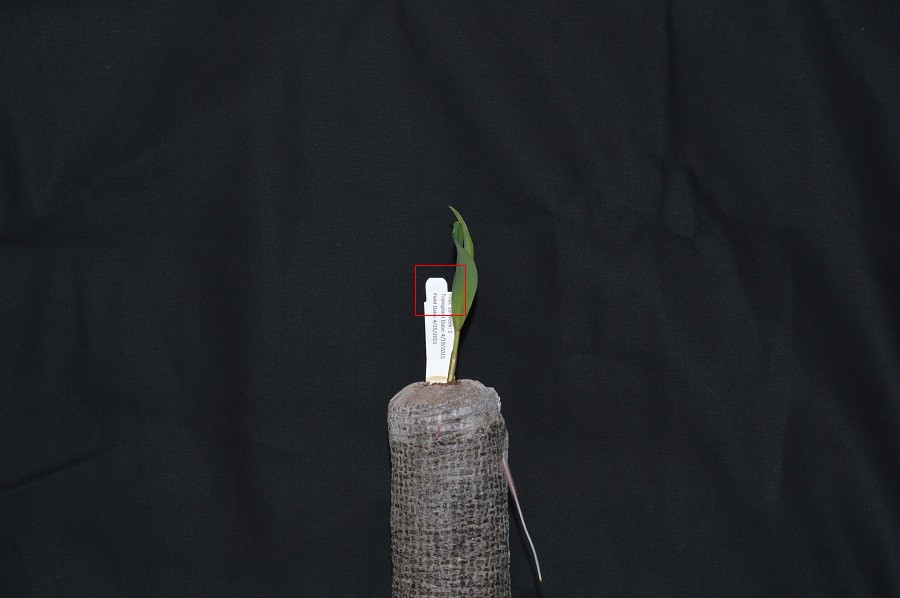
For example, consider this image of a maize seedling, with a square area designated by a red box:

Now, if we zoomed in close enough to see the pixels in the red box, we would see something like this:

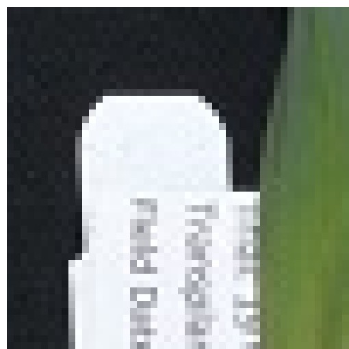
Note that each square in the enlarged image area - each pixel - is all one colour, but that each pixel can have a different colour from its neighbors. Viewed from a distance, these pixels seem to blend together to form the image we see.

Real-world images are typically made up of a vast number of pixels, and each of these pixels is one of potentially millions of colours. While we will deal with pictures of such complexity in this lesson, let’s start our exploration with just 15 pixels in a 5 x 3 matrix with 2 colours, and work our way up to that complexity.

Matrices, arrays, images and pixels

A matrix is a mathematical concept - numbers evenly arranged in a rectangle. This can be a two-dimensional rectangle, like the shape of the screen you’re looking at now. Or it could be a three-dimensional equivalent, a cuboid, or have even more dimensions, but always keeping the evenly spaced arrangement of numbers. In computing, an array refers to a structure in the computer’s memory where data is stored in evenly spaced elements. This is strongly analogous to a matrix. A NumPy array is a type of variable (a simpler example of a type is an integer). For our purposes, the distinction between matrices and arrays is not important, we don’t really care how the computer arranges our data in its memory. The important thing is that the computer stores values describing the pixels in images, as arrays. And the terms matrix and array will be used interchangeably.

Loading images

As noted, images we want to analyze (process) with Python are loaded into arrays. There are multiple ways to load images. In this lesson, we use imageio, a Python library for reading (loading) and writing (saving) image data, and more specifically its version 3. But, really, we could use any image loader which would return a NumPy array.

The v3 module of imageio (imageio.v3) is imported as iio (see note in the next section). Version 3 of imageio has the benefit of supporting nD (multidimensional) image data natively (think of volumes, movies).

"""Python library for reading and writing images."""

import imageio.v3 as iio

Let us load our image data from disk using the imread function from the imageio.v3 module.

Note that, using the same image loader or a different one, we could also read in remotely hosted data.

Why not use skimage.io.imread()?

The scikit-image library has its own function to read an image, so you might be asking why we don’t use it here. Actually, skimage.io.imread() uses iio.imread() internally when loading an image into Python. It is certainly something you may use as you see fit in your own code. In this lesson, we use the imageio library to read or write images, while scikit-image is dedicated to performing operations on the images. Using imageio gives us more flexibility, especially when it comes to handling metadata.

Beyond NumPy arrays

Beyond NumPy arrays, there exist other types of variables which are array-like. Notably, pandas.DataFrame and xarray.DataArray can hold labeled, tabular data. These are not natively supported in scikit-image, the scientific toolkit we use in this lesson for processing image data. However, data stored in these types can be converted to numpy.ndarray with certain assumptions (see pandas.DataFrame.to_numpy() and xarray.DataArray.data). Particularly, these conversions ignore the sampling coordinates (DataFrame.index, DataFrame.columns, or DataArray.coords), which may result in misrepresented data, for instance, when the original data points are irregularly spaced.

eight = iio.imread(uri="data/eight.tif")
print(type(eight))

<class 'numpy.ndarray'>

Working with pixels

First, let us add the necessary imports:

Import statements in Python

In Python, the import statement is used to load additional functionality into a program. This is necessary when we want our code to do something more specialised, which cannot easily be achieved with the limited set of basic tools and data structures available in the default Python environment.

Additional functionality can be loaded as a single function or object, a module defining several of these, or a library containing many modules. You will encounter several different forms of import statement.

import skimage                 # form 1, load whole skimage library
import skimage.draw            # form 2, load skimage.draw module only
from skimage.draw import disk  # form 3, load only the disk function
import skimage as ski          # form 4, load all of skimage into an object called ski

In the example above, form 1 loads the entire scikit-image library into the program as an object. Individual modules of the library are then available within that object, e.g., to access the disk function used in the drawing episode, you would write skimage.draw.disk().

Form 2 loads only the draw module of skimage into the program. The syntax needed to use the module remains unchanged: to access the disk function, we would use the same function call as given for form 1.

Form 3 can be used to import only a specific function/class from a library/module. Unlike the other forms, when this approach is used, the imported function or class can be called by its name only, without prefixing it with the name of the library/module from which it was loaded, i.e., disk() instead of skimage.draw.disk() using the example above. One hazard of this form is that importing like this will overwrite any object with the same name that was defined/imported earlier in the program, i.e., the example above would replace any existing object called disk with the disk function from skimage.draw.

Finally, the as keyword can be used when importing, to define a name to be used as shorthand for the library/module being imported. This name is referred to as an alias. Typically, using an alias (such as np for the NumPy library) saves us a little typing. You may see as combined with any of the other first three forms of import statements.

Which form is used often depends on the size and number of additional tools being loaded into the program.

Now that we have our libraries loaded, we will run a Jupyter Magic Command that will ensure our images display in our Jupyter document with pixel information that will help us more efficiently run commands later in the session.

"""Python libraries for learning and performing image processing."""

import ipympl
import matplotlib.pyplot as plt
import numpy as np
import skimage as ski

%matplotlib widget

With that taken care of, let us display the image we have loaded, using the imshow function from the matplotlib.pyplot module.

fig, ax = plt.subplots()
ax.imshow(eight)

<matplotlib.image.AxesImage at 0x7fb753eb2f10>

You might be thinking, “That does look vaguely like an eight, and I see two colours but how can that be only 15 pixels”. The display of the eight you see does use a lot more screen pixels to display our eight so large, but that does not mean there is information for all those screen pixels in the file. All those extra pixels are a consequence of our viewer creating additional pixels through interpolation. It could have just displayed it as a tiny image using only 15 screen pixels if the viewer was designed differently.

While many image file formats contain descriptive metadata that can be essential, the bulk of a picture file is just arrays of numeric information that, when interpreted according to a certain rule set, become recognizable as an image to us. Our image of an eight is no exception, and imageio.v3 stored that image data in an array of arrays making a 5 x 3 matrix of 15 pixels. We can demonstrate that by calling on the shape property of our image variable and see the matrix by printing our image variable to the screen.

print(eight.shape)
print(eight)

(5, 3)
[[0. 0. 0.]
 [0. 1. 0.]
 [0. 0. 0.]
 [0. 1. 0.]
 [0. 0. 0.]]

Thus if we have tools that will allow us to manipulate these arrays of numbers, we can manipulate the image. The NumPy library can be particularly useful here, so let’s try that out using NumPy array slicing. Notice that the default behavior of the imshow function appended row and column numbers that will be helpful to us as we try to address individual or groups of pixels. First let’s load another copy of our eight, and then make it look like a zero.

To make it look like a zero, we need to change the number underlying the centremost pixel to be 1. With the help of those row and column headers, at this small scale we can determine the centre pixel is in row labeled 2 and column labeled 1. Using array slicing, we can then address and assign a new value to that position.

zero = iio.imread(uri="data/eight.tif")
zero[2, 1] = 1.0

# The following line of code creates a new figure for imshow to use in displaying our output.
fig, ax = plt.subplots()
ax.imshow(zero)
print(zero)

[[0. 0. 0.]
 [0. 1. 0.]
 [0. 1. 0.]
 [0. 1. 0.]
 [0. 0. 0.]]

Coordinate system

When we process images, we can access, examine, and / or change the colour of any pixel we wish. To do this, we need some convention on how to access pixels individually; a way to give each one a name, or an address of a sort.

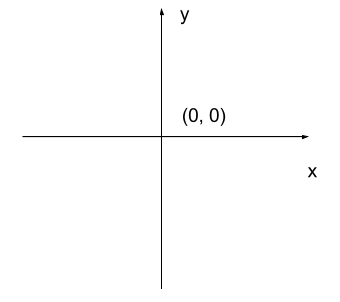
The most common manner to do this, and the one we will use in our programs, is to assign a modified Cartesian coordinate system to the image. The coordinate system we usually see in mathematics has a horizontal x-axis and a vertical y-axis, like this:

The modified coordinate system used for our images will have only positive coordinates, the origin will be in the upper left corner instead of the centre, and y coordinate values will get larger as they go down instead of up, like this:

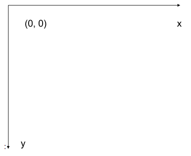
This is called a left-hand coordinate system. If you hold your left hand in front of your face and point your thumb at the floor, your extended index finger will correspond to the x-axis while your thumb represents the y-axis.

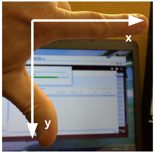
Until you have worked with images for a while, the most common mistake that you will make with coordinates is to forget that y coordinates get larger as they go down instead of up as in a normal Cartesian coordinate system. Consequently, it may be helpful to think in terms of counting down rows (r) for the y-axis and across columns (c) for the x-axis. This can be especially helpful in cases where you need to transpose image viewer data provided in x,y format to y,x format. Thus, we will use cx and ry where appropriate to help bridge these two approaches.

Exercise: Changing Pixel Values (5 min)

Load another copy of eight named five, and then change the value of pixels so you have what looks like a 5 instead of an 8. Display the image and print out the matrix as well.

Solution

There are many possible solutions, but one method would be …

five = iio.imread(uri="data/eight.tif")
five[1, 2] = 1.0
five[3, 0] = 1.0
fig, ax = plt.subplots()
ax.imshow(five)
print(five)

Output:

[[0. 0. 0.]
 [0. 1. 1.]
 [0. 0. 0.]
 [1. 1. 0.]
 [0. 0. 0.]]

More colours

Up to now, we only had a 2 colour matrix, but we can have more if we use other numbers or fractions. One common way is to use the numbers between 0 and 255 to allow for 256 different colours or 256 different levels of grey. Let’s try that out.

# make a copy of eight
three_colours = iio.imread(uri="data/eight.tif")

# multiply the whole matrix by 128
three_colours = three_colours * 128

# set the middle row (index 2) to the value of 255.,
# so you end up with the values 0., 128., and 255.
three_colours[2, :] = 255.
fig, ax = plt.subplots()
ax.imshow(three_colours)
print(three_colours)

[[  0.   0.   0.]
 [  0. 128.   0.]
 [255. 255. 255.]
 [  0. 128.   0.]
 [  0.   0.   0.]]

We now have 3 colours, but are they the three colours you expected? They all appear to be on a continuum of dark purple on the low end and yellow on the high end. This is a consequence of the default colour map (cmap) in this library. You can think of a colour map as an association or mapping of numbers to a specific colour. However, the goal here is not to have one number for every possible colour, but rather to have a continuum of colours that demonstrate relative intensity. In our specific case here for example, 255 or the highest intensity is mapped to yellow, and 0 or the lowest intensity is mapped to a dark purple. The best colour map for your data will vary and there are many options built in, but this default selection was not arbitrary. A lot of science went into making this the default due to its robustness when it comes to how the human mind interprets relative colour values, grey-scale printability, and colour-blind friendliness (You can read more about this default colour map in a Matplotlib tutorial and an explanatory article by the authors). Thus it is a good place to start, and you should change it only with purpose and forethought. For now, let’s see how you can do that using an alternative map you have likely seen before where it will be even easier to see it as a mapped continuum of intensities: greyscale.

fig, ax = plt.subplots()
ax.imshow(three_colours, cmap="gray")

<matplotlib.image.AxesImage at 0x7fb753afce50>

Above we have exactly the same underlying data matrix, but in greyscale. Zero maps to black, 255 maps to white, and 128 maps to medium grey. Here we only have a single channel in the data and utilize a grayscale color map to represent the luminance, or intensity of the data and correspondingly this channel is referred to as the luminance channel.

Even more colours

This is all well and good at this scale, but what happens when we instead have a picture of a natural landscape that contains millions of colours. Having a one to one mapping of number to colour like this would be inefficient and make adjustments and building tools to do so very difficult. Rather than larger numbers, the solution is to have more numbers in more dimensions. Storing the numbers in a multi-dimensional matrix where each colour or property like transparency is associated with its own dimension allows for individual contributions to a pixel to be adjusted independently. This ability to manipulate properties of groups of pixels separately will be key to certain techniques explored in later chapters of this lesson. To get started let’s see an example of how different dimensions of information combine to produce a set of pixels using a 4 x 4 matrix with 3 dimensions for the colours red, green, and blue. Rather than loading it from a file, we will generate this example using NumPy.

# set the random seed so we all get the same matrix
pseudorandomizer = np.random.RandomState(2021)
# create a 4 × 4 checkerboard of random colours
checkerboard = pseudorandomizer.randint(0, 255, size=(4, 4, 3))
# restore the default map as you show the image
fig, ax = plt.subplots()
ax.imshow(checkerboard)
# display the arrays
print(checkerboard)

[[[116  85  57]
  [128 109  94]
  [214  44  62]
  [219 157  21]]

 [[ 93 152 140]
  [246 198 102]
  [ 70  33 101]
  [  7   1 110]]

 [[225 124 229]
  [154 194 176]
  [227  63  49]
  [144 178  54]]

 [[123 180  93]
  [120   5  49]
  [166 234 142]
  [ 71  85  70]]]

Previously we had one number being mapped to one colour or intensity. Now we are combining the effect of 3 numbers to arrive at a single colour value. Let’s see an example of that using the blue square at the end of the second row, which has the index [1, 3].

# extract all the colour information for the blue square
upper_right_square = checkerboard[1, 3, :]
upper_right_square

array([  7,   1, 110])

This outputs: array([  7,   1, 110]) The integers in order represent Red, Green, and Blue. Looking at the 3 values and knowing how they map, can help us understand why it is blue. If we divide each value by 255, which is the maximum, we can determine how much it is contributing relative to its maximum potential. Effectively, the red is at 7/255 or 2.8 percent of its potential, the green is at 1/255 or 0.4 percent, and blue is 110/255 or 43.1 percent of its potential. So when you mix those three intensities of colour, blue is winning by a wide margin, but the red and green still contribute to make it a slightly different shade of blue than 0,0,110 would be on its own.

These colours mapped to dimensions of the matrix may be referred to as channels. It may be helpful to display each of these channels independently, to help us understand what is happening. We can do that by multiplying our image array representation with a 1d matrix that has a one for the channel we want to keep and zeros for the rest.

red_channel = checkerboard * [1, 0, 0]
fig, ax = plt.subplots()
ax.imshow(red_channel)

green_channel = checkerboard * [0, 1, 0]
fig, ax = plt.subplots()
ax.imshow(green_channel)

blue_channel = checkerboard * [0, 0, 1]
fig, ax = plt.subplots()
ax.imshow(blue_channel)

<matplotlib.image.AxesImage at 0x7fb75174e150>

If we look at the upper [1, 3] square in all three figures, we can see each of those colour contributions in action. Notice that there are several squares in the blue figure that look even more intensely blue than square [1, 3]. When all three channels are combined though, the blue light of those squares is being diluted by the relative strength of red and green being mixed in with them.

24-bit RGB colour

This last colour model we used, known as the RGB (Red, Green, Blue) model, is the most common.

As we saw, the RGB model is an additive colour model, which means that the primary colours are mixed together to form other colours. Most frequently, the amount of the primary colour added is represented as an integer in the closed range [0, 255] as seen in the example. Therefore, there are 256 discrete amounts of each primary colour that can be added to produce another colour. The number of discrete amounts of each colour, 256, corresponds to the number of bits used to hold the colour channel value, which is eight (2⁸=256). Since we have three channels with 8 bits for each (8+8+8=24), this is called 24-bit colour depth.

Any particular colour in the RGB model can be expressed by a triplet of integers in [0, 255], representing the red, green, and blue channels, respectively. A larger number in a channel means that more of that primary colour is present.

Exercise: Thinking about RGB colours (5 min)

Suppose that we represent colours as triples (r, g, b), where each of r, g, and b is an integer in [0, 255]. What colours are represented by each of these triples? (Try to answer these questions without reading further.)

1. (255, 0, 0)

2. (0, 255, 0)

3. (0, 0, 255)

4. (255, 255, 255)

5. (0, 0, 0)

6. (128, 128, 128)

Solution

1. (255, 0, 0) represents red, because the red channel is maximised, while the other two channels have the minimum values.

2. (0, 255, 0) represents green.

3. (0, 0, 255) represents blue.

4. (255, 255, 255) — when we mix the maximum value of all three colour channels, we see white.

5. (0, 0, 0) represents the absence of all colour, or black.

6. (128, 128, 128) represents a medium shade of gray. Note that the 24-bit RGB colour model provides at least 254 shades of gray, rather than only fifty.

Note that the RGB colour model may run contrary to your experience, especially if you have mixed primary colours of paint to create new colours. In the RGB model, the lack of any colour is black, while the maximum amount of each of the primary colours is white.

After completing the previous challenge, we can look at some further examples of 24-bit RGB colours, in a visual way. The image in the next challenge shows some colour names, their 24-bit RGB triplet values, and the colour itself.

Exercise: RGB colour table (optional)

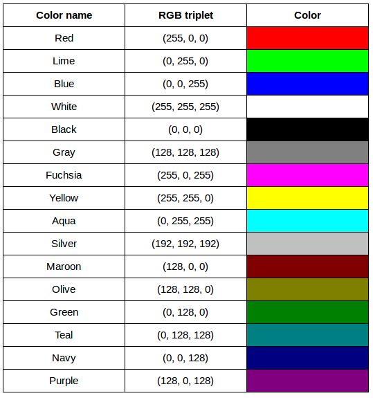
We cannot really provide a complete table. To see why, answer this question: How many possible colours can be represented with the 24-bit RGB model?

Solution

There are 24 total bits in an RGB colour of this type, and each bit can be on or off, and so there are 2²⁴ = 16,777,216 possible colours with our additive, 24-bit RGB colour model.

Although 24-bit colour depth is common, there are other options. For example, we might have 8-bit colour (3 bits for red and green, but only 2 for blue, providing 8 × 8 × 4 = 256 colours) or 16-bit colour (4 bits for red, green, and blue, plus 4 more for transparency, providing 16 × 16 × 16 = 4096 colours, with 16 transparency levels each). There are colour depths with more than eight bits per channel, but as the human eye can only discern approximately 10 million different colours, these are not often used.

If you are using an older or inexpensive laptop screen or LCD monitor to view images, it may only support 18-bit colour, capable of displaying 64 × 64 × 64 = 262,144 colours. 24-bit colour images will be converted in some manner to 18-bit, and thus the colour quality you see will not match what is actually in the image.

We can combine our coordinate system with the 24-bit RGB colour model to gain a conceptual understanding of the images we will be working with. An image is a rectangular array of pixels, each with its own coordinate. Each pixel in the image is a square point of coloured light, where the colour is specified by a 24-bit RGB triplet. Such an image is an example of raster graphics.

Image formats

Although the images we will manipulate in our programs are conceptualised as rectangular arrays of RGB triplets, they are not necessarily created, stored, or transmitted in that format. There are several image formats we might encounter, and we should know the basics of at least a few of them. Some formats we might encounter, and their file extensions, are shown in this table:

Format	Extension
Device-Independent Bitmap (BMP)	.bmp
Joint Photographic Experts Group (JPEG)	.jpg or .jpeg
Tagged Image File Format (TIFF)	.tif or .tiff

BMP

The file format that comes closest to our preceding conceptualisation of images is the Device-Independent Bitmap, or BMP, file format. BMP files store raster graphics images as long sequences of binary-encoded numbers that specify the colour of each pixel in the image. Since computer files are one-dimensional structures, the pixel colours are stored one row at a time. That is, the first row of pixels (those with y-coordinate 0) are stored first, followed by the second row (those with y-coordinate 1), and so on. Depending on how it was created, a BMP image might have 8-bit, 16-bit, or 24-bit colour depth.

24-bit BMP images have a relatively simple file format, can be viewed and loaded across a wide variety of operating systems, and have high quality. However, BMP images are not compressed, resulting in very large file sizes for any useful image resolutions.

The idea of image compression is important to us for two reasons: first, compressed images have smaller file sizes, and are therefore easier to store and transmit; and second, compressed images may not have as much detail as their uncompressed counterparts, and so our programs may not be able to detect some important aspect if we are working with compressed images. Since compression is important to us, we should take a brief detour and discuss the concept.

Image compression

Before discussing additional formats, familiarity with image compression will be helpful. Let’s delve into that subject with a challenge. For this challenge, you will need to know about bits / bytes and how those are used to express computer storage capacities. If you already know, you can skip to the challenge below.

Bits and bytes

Before we talk specifically about images, we first need to understand how numbers are stored in a modern digital computer. When we think of a number, we do so using a decimal, or base-10 place-value number system. For example, a number like 659 is 6 × 10² + 5 × 10¹ + 9 × 10⁰. Each digit in the number is multiplied by a power of 10, based on where it occurs, and there are 10 digits that can occur in each position (0, 1, 2, 3, 4, 5, 6, 7, 8, 9).

In principle, computers could be constructed to represent numbers in exactly the same way. But, the electronic circuits inside a computer are much easier to construct if we restrict the numeric base to only two, instead of 10. So, values in a computer are stored using a binary, or base-2 place-value number system.

In this system, each symbol in a number is called a bit instead of a digit, and there are only two values for each bit (0 and 1). We might imagine a four-bit binary number, 1101. Using the same kind of place-value expansion as we did above for 659, we see that 1101 = 1 × 2³ + 1 × 2² + 0 × 2¹ + 1 × 2⁰, which if we do the math is 8 + 4 + 0 + 1, or 13 in decimal.

Internally, computers have a minimum number of bits that they work with at a given time: eight. A group of eight bits is called a byte. The amount of memory (RAM) and drive space our computers have is quantified by terms like Megabytes (MB), Gigabytes (GB), and Terabytes (TB). The following table provides more formal definitions for these terms.

Unit	Abbreviation	Size
Kilobyte	KB	1024 bytes
Megabyte	MB	1024 KB
Gigabyte	GB	1024 MB
Terabyte	TB	1024 GB

Exercise: BMP image size (optional)

Imagine that we have a fairly large, but very boring image: a 5,000 × 5,000 pixel image composed of nothing but white pixels. If we used an uncompressed image format such as BMP, with the 24-bit RGB colour model, how much storage would be required for the file?

Solution

In such an image, there are 5,000 × 5,000 = 25,000,000 pixels, and 24 bits for each pixel, leading to 25,000,000 × 24 = 600,000,000 bits, or 75,000,000 bytes (71.5MB). That is quite a lot of space for a very uninteresting image!

Since image files can be very large, various compression schemes exist for saving (approximately) the same information while using less space. These compression techniques can be categorised as lossless or lossy.

Lossless compression

In lossless image compression, we apply some algorithm (i.e., a computerised procedure) to the image, resulting in a file that is significantly smaller than the uncompressed BMP file equivalent would be. Then, when we wish to load and view or process the image, our program reads the compressed file, and reverses the compression process, resulting in an image that is identical to the original. Nothing is lost in the process – hence the term “lossless.”

The general idea of lossless compression is to somehow detect long patterns of bytes in a file that are repeated over and over, and then assign a smaller bit pattern to represent the longer sample. Then, the compressed file is made up of the smaller patterns, rather than the larger ones, thus reducing the number of bytes required to save the file. The compressed file also contains a table of the substituted patterns and the originals, so when the file is decompressed it can be made identical to the original before compression.

To provide you with a concrete example, consider the 71.5 MB white BMP image discussed above. When put through the zip compression utility on Microsoft Windows, the resulting .zip file is only 72 KB in size! That is, the .zip version of the image is three orders of magnitude smaller than the original, and it can be decompressed into a file that is byte-for-byte the same as the original. Since the original is so repetitious - simply the same colour triplet repeated 25,000,000 times - the compression algorithm can dramatically reduce the size of the file.

If you work with .zip or .gz archives, you are dealing with lossless compression.

Lossy compression

Lossy compression takes the original image and discards some of the detail in it, resulting in a smaller file format. The goal is to only throw away detail that someone viewing the image would not notice. Many lossy compression schemes have adjustable levels of compression, so that the image creator can choose the amount of detail that is lost. The more detail that is sacrificed, the smaller the image files will be - but of course, the detail and richness of the image will be lower as well.

This is probably fine for images that are shown on Web pages or printed off on 4 × 6 photo paper, but may or may not be fine for scientific work. You will have to decide whether the loss of image quality and detail are important to your work, versus the space savings afforded by a lossy compression format.

It is important to understand that once an image is saved in a lossy compression format, the lost detail is just that - lost. I.e., unlike lossless formats, given an image saved in a lossy format, there is no way to reconstruct the original image in a byte-by-byte manner.

JPEG

A common image format is JPEG, which is often used for photographs. JPEG images are lossy. When a JPEG image is saved, some of the detail is thrown away. The larger the compression, the more detail is thrown away.

JPEG images are often used in websites and email because of their small file sizes. They are also used in digital cameras because they allow for a large number of photographs to be stored on a memory card.

Exercise: Examining actual image sizes (optional)

Let’s see how much space our image files actually use. First, make a 5,000 × 5,000 pixel pure white image using NumPy, save it as a BMP file called ws.bmp, and then save it again as a JPEG file called ws.jpg. How large are the two files?

Solution

Here is a Python program to create the white image and save it in BMP and JPEG formats.

import imageio.v3 as iio
import numpy as np

# Create a 5000 x 5000 white image
white = np.zeros(shape=(5000, 5000, 3), dtype="uint8")
white.fill(255)

# Save as BMP and JPEG
iio.imwrite(uri="ws.bmp", image=white)
iio.imwrite(uri="ws.jpg", image=white)

The BMP file should be around 71.5 MB, while the JPEG file should be much smaller, perhaps only a few hundred kilobytes.

Exercise: Comparing lossless versus lossy compression (optional)

Let us see the effects of lossy compression on image quality. Using the original image data/eight.tif, save a copy as a JPEG file, and then reload both images and compare them. What differences do you notice?

Solution

Here is a Python program that loads the original image, saves a JPEG copy, and then reloads both:

import imageio.v3 as iio
import numpy as np
import skimage

original = iio.imread(uri="data/eight.tif")
iio.imwrite(uri="data/eight.jpg", image=original)
jpeg_copy = iio.imread(uri="data/eight.jpg")

# Check if the images are identical
print(np.array_equal(original, jpeg_copy))

# Compute the difference
difference = skimage.util.compare_images(original, jpeg_copy, method="diff")

The comparison will show that the images are NOT identical. The JPEG compression process has changed some pixel values slightly.

Now let’s visualise the effects of JPEG compression quality on an image. Lossy compression algorithms often allow us to specify how much detail we are willing to sacrifice in exchange for smaller file sizes. The following images show the same photograph saved with different JPEG quality settings:

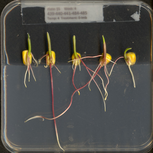
The original image.

The image saved as a TIFF with lossless compression.

The image saved with JPEG compression.

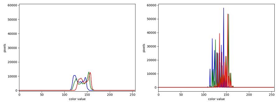
Histogram showing differences between the TIFF and JPEG versions.

The difference between the TIFF and JPEG versions may not be obvious at a glance, but the histogram clearly shows that the JPEG version has lost some detail.

PNG

Portable Network Graphics (PNG) images are lossless. PNG is a lossless format that can faithfully reproduce the original image. PNG images support higher colour depths than some other formats, and are commonly used on websites where small file sizes are important but image quality must be preserved.

PNG images use a row-oriented storage structure combined with a filtering step that makes the subsequent lossless compression more effective. Images with large regions of uniform colour compress particularly well as PNG.

TIFF

Tagged Image File Format (TIFF) images are used by publishers and graphic designers, as well as by scientists. TIFF images can be stored using lossless or lossy compression, or with no compression at all. TIFF images are popular because they support a wide range of colour depths, from 1-bit black and white through to 32-bit full colour images.

TIFF images may also store metadata - text fields that describe the image in some way. This metadata can include things like the make and model of the camera used to take a photo, the date and time when the photo was taken, the GPS coordinates where the photo was taken, and more.

Metadata

JPEG and TIFF images support the embedding of metadata, i.e., textual information stored inside the image file itself. When a Python program reads a JPEG or TIFF file into a NumPy array, the metadata is not included in the array; it is discarded during the reading process. Conversely, when imageio.v3 writes a NumPy array as a JPEG or TIFF image file, the program cannot determine what metadata should be included with the image, and so no metadata will be written. If metadata is important to your work, take care when reading and writing images!

Accessing metadata

We can read the metadata from an image file without reading the image itself. Here is how to do this using imageio.v3:

import imageio.v3 as iio
metadata = iio.immeta(uri="data/eight.tif")
print(metadata)

The output might look something like this:

{'is_fluoview': False, 'is_nih': False, 'is_micromanager': False,
 'is_ome': False, 'is_lsm': False, 'is_shaped': True, 'is_stk': False,
 'is_svs': False, 'is_mdgel': False, 'is_mediacy': False,
 'is_reduced': False, 'is_mask': False, 'axes': 'YXS', ...}

Different image formats and files will contain different metadata.

Here is a table that summarises the characteristics of the BMP, JPEG, PNG, and TIFF image formats:

Format	Compression	Metadata	Advantages	Disadvantages
BMP	None	None	High quality; universal support	Very large file sizes
JPEG	Lossy	Yes	Small file sizes	Detail lost; not suitable for repeated save/reload
PNG	Lossless	None	Lossless; good for web; supports transparency	Larger files than JPEG; no metadata
TIFF	None, lossless, or lossy	Yes	Flexible; supports wide range of colour depths and metadata	Can be very large; not universally supported

Summary Quiz