Thresholding

Questions

• How can we use thresholding to produce a binary image?

Objectives

• Explain what thresholding is and how it can be used.

• Use histograms to determine appropriate threshold values to use for the thresholding process.

• Apply simple, fixed-level binary thresholding to an image.

• Explain the difference between using the operator > or the operator < to threshold an image represented by a NumPy array.

• Describe the shape of a binary image produced by thresholding via > or <.

• Explain when Otsu’s method for automatic thresholding is appropriate.

• Apply automatic thresholding to an image using Otsu’s method.

• Use the np.count_nonzero() function to count the number of non-zero pixels in an image.

In this episode, we will learn how to use scikit-image functions to apply thresholding to an image. Thresholding is a type of image segmentation, where we change the pixels of an image to make the image easier to analyze. In thresholding, we convert an image from colour or grayscale into a binary image, i.e., one that is simply black and white. Most frequently, we use thresholding as a way to select areas of interest of an image, while ignoring the parts we are not concerned with. We have already done some simple thresholding, in the “Manipulating pixels” section of the Working with scikit-image episode. In that case, we used a simple NumPy array manipulation to separate the pixels belonging to the root system of a plant from the black background. In this episode, we will learn how to use scikit-image functions to perform thresholding. Then, we will use the masks returned by these functions to select the parts of an image we are interested in.

First, import the packages needed for this episode

import glob

import imageio.v3 as iio
import ipympl
import matplotlib.pyplot as plt
import numpy as np
import skimage as ski

%matplotlib widget

Simple thresholding

Consider the image data/shapes-01.jpg with a series of crudely cut shapes set against a white background.

# load the image
shapes01 = iio.imread(uri="data/shapes-01.jpg")

fig, ax = plt.subplots()
ax.imshow(shapes01)

<matplotlib.image.AxesImage at 0x7fd21859e750>

Now suppose we want to select only the shapes from the image. In other words, we want to leave the pixels belonging to the shapes “on,” while turning the rest of the pixels “off,” by setting their colour channel values to zeros. The scikit-image library has several different methods of thresholding. We will start with the simplest version, which involves an important step of human input. Specifically, in this simple, fixed-level thresholding, we have to provide a threshold value t.

The process works like this. First, we will load the original image, convert it to grayscale, and de-noise it as in the Blurring Images episode.

# convert the image to grayscale
gray_shapes = ski.color.rgb2gray(shapes01)

# blur the image to denoise
blurred_shapes = ski.filters.gaussian(gray_shapes, sigma=1.0)

fig, ax = plt.subplots()
ax.imshow(blurred_shapes, cmap="gray")

<matplotlib.image.AxesImage at 0x7fd218063490>

Next, we would like to apply the threshold t such that pixels with grayscale values on one side of t will be turned “on”, while pixels with grayscale values on the other side will be turned “off”. How might we do that? Remember that grayscale images contain pixel values in the range from 0 to 1, so we are looking for a threshold t in the closed range [0.0, 1.0]. We see in the image that the geometric shapes are “darker” than the white background but there is also some light gray noise on the background. One way to determine a “good” value for t is to look at the grayscale histogram of the image and try to identify what grayscale ranges correspond to the shapes in the image or the background.

The histogram for the shapes image shown above can be produced as in the Creating Histograms episode.

# create a histogram of the blurred grayscale image
histogram, bin_edges = np.histogram(blurred_shapes, bins=256, range=(0.0, 1.0))

fig, ax = plt.subplots()
ax.plot(bin_edges[0:-1], histogram)
ax.set_title("Grayscale Histogram")
ax.set_xlabel("grayscale value")
ax.set_ylabel("pixels")
ax.set_xlim(0, 1.0)

(0.0, 1.0)

Since the image has a white background, most of the pixels in the image are white. This corresponds nicely to what we see in the histogram: there is a peak near the value of 1.0. If we want to select the shapes and not the background, we want to turn off the white background pixels, while leaving the pixels for the shapes turned on. So, we should choose a value of t somewhere before the large peak and turn pixels above that value “off”. Let us choose t=0.8.

To apply the threshold t, we can use the NumPy comparison operators to create a mask. Here, we want to turn “on” all pixels which have values smaller than the threshold, so we use the less operator < to compare the blurred_image to the threshold t. The operator returns a mask, that we capture in the variable binary_mask. It has only one channel, and each of its values is either 0 or 1. The binary mask created by the thresholding operation can be shown with ax.imshow, where the False entries are shown as black pixels (0-valued) and the True entries are shown as white pixels (1-valued).

# create a mask based on the threshold
t = 0.8
binary_mask = blurred_shapes < t

fig, ax = plt.subplots()
ax.imshow(binary_mask, cmap="gray")

<matplotlib.image.AxesImage at 0x7fd200768a50>

You can see that the areas where the shapes were in the original area are now white, while the rest of the mask image is black.

What makes a good threshold?

As is often the case, the answer to this question is “it depends”. In the example above, we could have just switched off all the white background pixels by choosing t=1.0, but this would leave us with some background noise in the mask image. On the other hand, if we choose too low a value for the threshold, we could lose some of the shapes that are too bright. You can experiment with the threshold by re-running the above code lines with different values for t. In practice, it is a matter of domain knowledge and experience to interpret the peaks in the histogram so to determine an appropriate threshold. The process often involves trial and error, which is a drawback of the simple thresholding method. Below we will introduce automatic thresholding, which uses a quantitative, mathematical definition for a good threshold that allows us to determine the value of t automatically. It is worth noting that the principle for simple and automatic thresholding can also be used for images with pixel ranges other than [0.0, 1.0]. For example, we could perform thresholding on pixel intensity values in the range [0, 255] as we have already seen in the Working with scikit-image episode.

We can now apply the binary_mask to the original coloured image as we have learned in the Drawing and Bitwise Operations episode. What we are left with is only the coloured shapes from the original.

# use the binary_mask to select the "interesting" part of the image
selection = shapes01.copy()
selection[~binary_mask] = 0

fig, ax = plt.subplots()
ax.imshow(selection)

<matplotlib.image.AxesImage at 0x7fd20078b990>

Exercise: More practice with simple thresholding (15 min)

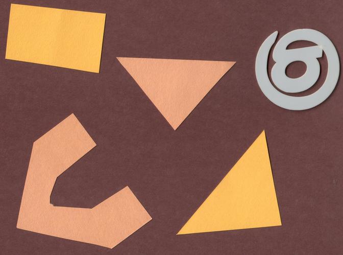
Now, it is your turn to practice. Suppose we want to use simple thresholding to select only the coloured shapes (in this particular case we consider grayish to be a colour, too) from the image data/shapes-02.jpg:

First, plot the grayscale histogram as in the Creating Histogram episode and examine the distribution of grayscale values in the image. What do you think would be a good value for the threshold t?

Solution

The histogram for the data/shapes-02.jpg image can be shown with

shapes = iio.imread(uri="data/shapes-02.jpg")
gray_shapes = ski.color.rgb2gray(shapes)
histogram, bin_edges = np.histogram(gray_shapes, bins=256, range=(0.0, 1.0))

fig, ax = plt.subplots()
ax.plot(bin_edges[0:-1], histogram)
ax.set_title("Graylevel histogram")
ax.set_xlabel("gray value")
ax.set_ylabel("pixel count")
ax.set_xlim(0, 1.0)

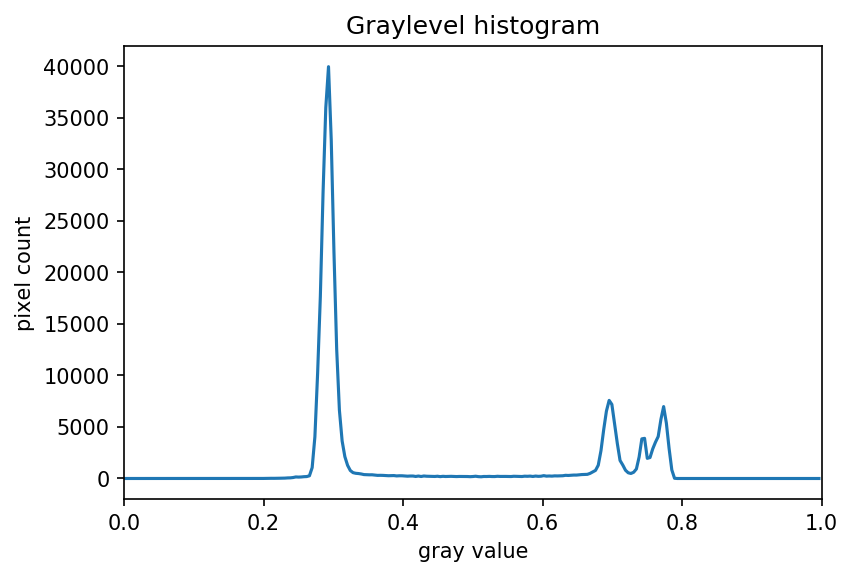
We can see a large spike around 0.3, and a smaller spike around 0.7. The spike near 0.3 represents the darker background, so it seems like a value close to t=0.5 would be a good choice.

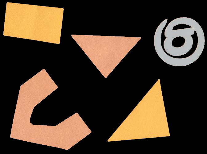
Next, create a mask to turn the pixels above the threshold t on and pixels below the threshold t off. Note that unlike the image with a white background we used above, here the peak for the background colour is at a lower gray level than the shapes. Therefore, change the comparison operator less < to greater > to create the appropriate mask. Then apply the mask to the image and view the thresholded image. If everything works as it should, your output should show only the coloured shapes on a black background.

Here are the commands to create and view the binary mask:

t = 0.5
binary_mask = gray_shapes > t

fig, ax = plt.subplots()
ax.imshow(binary_mask, cmap="gray")

And here are the commands to apply the mask and view the thresholded image:

shapes02 = iio.imread(uri="data/shapes-02.jpg")
selection = shapes02.copy()
selection[~binary_mask] = 0

fig, ax = plt.subplots()
ax.imshow(selection)

Automatic thresholding

The downside of the simple thresholding technique is that we have to make an educated guess about the threshold t by inspecting the histogram. There are also automatic thresholding methods that can determine the threshold automatically for us. One such method is Otsu’s method. It is particularly useful for situations where the grayscale histogram of an image has two peaks that correspond to background and objects of interest.

Denoising an image before thresholding

In practice, it is often necessary to denoise the image before thresholding, which can be done with one of the methods from the Blurring Images episode.

Consider the image data/maize-root-cluster.jpg of a maize root system which we have seen before in the Working with scikit-image episode.

maize_roots = iio.imread(uri="data/maize-root-cluster.jpg")

fig, ax = plt.subplots()
ax.imshow(maize_roots)

<matplotlib.image.AxesImage at 0x7fd2001b6950>

We use Gaussian blur with a sigma of 1.0 to denoise the root image. Let us look at the grayscale histogram of the denoised image.

# convert the image to grayscale
gray_image = ski.color.rgb2gray(maize_roots)

# blur the image to denoise
blurred_image = ski.filters.gaussian(gray_image, sigma=1.0)

# show the histogram of the blurred image
histogram, bin_edges = np.histogram(blurred_image, bins=256, range=(0.0, 1.0))
fig, ax = plt.subplots()
ax.plot(bin_edges[0:-1], histogram)
ax.set_title("Graylevel histogram")
ax.set_xlabel("gray value")
ax.set_ylabel("pixel count")
ax.set_xlim(0, 1.0)

(0.0, 1.0)

The histogram has a significant peak around 0.2 and then a broader “hill” around 0.6 followed by a smaller peak near 1.0. Looking at the grayscale image, we can identify the peak at 0.2 with the background and the broader peak with the foreground. Thus, this image is a good candidate for thresholding with Otsu’s method. The mathematical details of how this works are complicated (see the scikit-image documentation if you are interested), but the outcome is that Otsu’s method finds a threshold value between the two peaks of a grayscale histogram which might correspond well to the foreground and background depending on the data and application.

The ski.filters.threshold_otsu() function can be used to determine the threshold automatically via Otsu’s method. Then NumPy comparison operators can be used to apply it as before. Here are the Python commands to determine the threshold t with Otsu’s method.

# perform automatic thresholding
t = ski.filters.threshold_otsu(blurred_image)
print("Found automatic threshold t = {}.".format(t))

Found automatic threshold t = 0.4116003928683858.

For this root image and a Gaussian blur with the chosen sigma of 1.0, the computed threshold value is 0.42. Now we can create a binary mask with the comparison operator >. As we have seen before, pixels above the threshold value will be turned on, those below the threshold will be turned off.

# create a binary mask with the threshold found by Otsu's method
binary_mask = blurred_image > t

fig, ax = plt.subplots()
ax.imshow(binary_mask, cmap="gray")

<matplotlib.image.AxesImage at 0x7fd1ffbcac10>

Finally, we use the mask to select the foreground:

# apply the binary mask to select the foreground
selection = maize_roots.copy()
selection[~binary_mask] = 0

fig, ax = plt.subplots()
ax.imshow(selection)

<matplotlib.image.AxesImage at 0x7fd1f47912d0>

Application: measuring root mass

Let us now turn to an application where we can apply thresholding and other techniques we have learned to this point. Consider these four maize root system images, which you can find in the files data/trial-016.jpg, data/trial-020.jpg, data/trial-216.jpg, and data/trial-293.jpg.

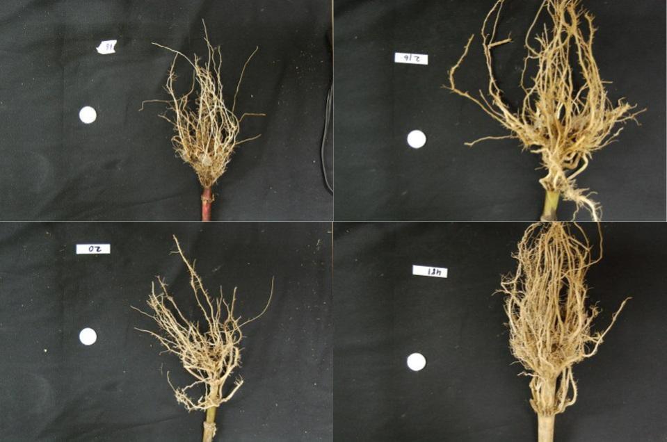
Suppose we are interested in the amount of plant material in each image, and in particular how that amount changes from image to image. Perhaps the images represent the growth of the plant over time, or perhaps the images show four different maize varieties at the same phase of their growth. The question we would like to answer is, “how much root mass is in each image?”

We will first construct a Python program to measure this value for a single image. Our strategy will be this:

1. Read the image, converting it to grayscale as it is read. For this application we do not need the colour image.

2. Blur the image.

3. Use Otsu’s method of thresholding to create a binary image, where the pixels that were part of the maize plant are white, and everything else is black.

4. Save the binary image so it can be examined later.

5. Count the white pixels in the binary image, and divide by the number of pixels in the image. This ratio will be a measure of the root mass of the plant in the image.

6. Output the name of the image processed and the root mass ratio.

Our intent is to perform these steps and produce the numeric result - a measure of the root mass in the image - without human intervention. Implementing the steps within a Python function will enable us to call this function for different images.

Here is a Python function that implements this root-mass-measuring strategy. Since the function is intended to produce numeric output without human interaction, it does not display any of the images. Almost all of the commands should be familiar, and in fact, it may seem simpler than the code we have worked on thus far, because we are not displaying any of the images.

def measure_root_mass(filename, sigma=1.0):

    # read the original image, converting to grayscale on the fly
    image = iio.imread(uri=filename, mode="L")

    # blur before thresholding
    blurred_image = ski.filters.gaussian(image, sigma=sigma)

    # perform automatic thresholding to produce a binary image
    t = ski.filters.threshold_otsu(blurred_image)
    binary_mask = blurred_image > t

    # determine root mass ratio
    root_pixels = np.count_nonzero(binary_mask)
    w = binary_mask.shape[1]
    h = binary_mask.shape[0]
    density = root_pixels / (w * h)

    return density

The function begins with reading the original image from the file filename. We use iio.imread() with the optional argument mode="L" to automatically convert it to grayscale. Next, the grayscale image is blurred with a Gaussian filter with the value of sigma that is passed to the function. Then we determine the threshold t with Otsu’s method and create a binary mask just as we did in the previous section. Up to this point, everything should be familiar.

The final part of the function determines the root mass ratio in the image. Recall that in the binary_mask, every pixel has either a value of zero (black/background) or one (white/foreground). We want to count the number of white pixels, which can be accomplished with a call to the NumPy function np.count_nonzero. Then we determine the width and height of the image by using the elements of binary_mask.shape (that is, the dimensions of the NumPy array that stores the image). Finally, the density ratio is calculated by dividing the number of white pixels by the total number of pixels w*h in the image. The function returns then root density of the image.

We can call this function with any filename and provide a sigma value for the blurring. If no sigma value is provided, the default value 1.0 will be used. For example, for the file data/trial-016.jpg and a sigma value of 1.5, we would call the function like this:

measure_root_mass(filename="data/trial-016.jpg", sigma=1.5)

0.04907247340425532

Now we can use the function to process the series of four images shown above. In a real-world scientific situation, there might be dozens, hundreds, or even thousands of images to process. To save us the tedium of calling the function for each image by hand, we can write a loop that processes all files automatically. The following code block assumes that the files are located in the same directory and the filenames all start with the trial- prefix and end with the .jpg suffix.

all_files = glob.glob("data/trial-*.jpg")
for filename in all_files:
    density = measure_root_mass(filename=filename, sigma=1.5)
    # output in format suitable for .csv
    print(filename, density, sep=",")

data/trial-016.jpg,0.04907247340425532

data/trial-020.jpg,0.06381366356382978

data/trial-293.jpg,0.13665791223404256

data/trial-216.jpg,0.14205152925531914

Exercise: Ignoring more of the images – brainstorming (10 min)

Let us take a closer look at the binary masks produced by the measure_root_mass function.

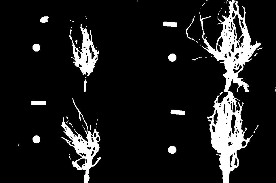
You may have noticed in the section on automatic thresholding that the thresholded image does include regions of the image aside of the plant root: the numbered labels and the white circles in each image are preserved during the thresholding, because their grayscale values are above the threshold. Therefore, our calculated root mass ratios include the white pixels of the label and white circle that are not part of the plant root. Those extra pixels affect how accurate the root mass calculation is!

How might we remove the labels and circles before calculating the ratio, so that our results are more accurate? Think about some options given what we have learned so far.

Solution

One approach we might take is to try to completely mask out a region from each image, particularly, the area containing the white circle and the numbered label. If we had coordinates for a rectangular area on the image that contained the circle and the label, we could mask the area out by using techniques we learned in the Drawing and Bitwise Operations episode.

However, a closer inspection of the binary images raises some issues with that approach. Since the roots are not always constrained to a certain area in the image, and since the circles and labels are in different locations each time, we would have difficulties coming up with a single rectangle that would work for every image. We could create a different masking rectangle for each image, but that is not a practicable approach if we have hundreds or thousands of images to process.

Another approach we could take is to apply two thresholding steps to the image. Look at the graylevel histogram of the file data/trial-016.jpg shown above again: Notice the peak near 1.0? Recall that a grayscale value of 1.0 corresponds to white pixels: the peak corresponds to the white label and circle. So, we could use simple binary thresholding to mask the white circle and label from the image, and then we could use Otsu’s method to select the pixels in the plant portion of the image.

Note that most of this extra work in processing the image could have been avoided during the experimental design stage, with some careful consideration of how the resulting images would be used. For example, all of the following measures could have made the images easier to process, by helping us predict and/or detect where the label is in the image and subsequently mask it from further processing:

• Using labels with a consistent size and shape

• Placing all the labels in the same position, relative to the sample

• Using a non-white label, with non-black writing

Exercise: Ignoring more of the images – implementation (30 min - optional, not included in timing)

Implement an enhanced version of the function measure_root_mass that applies simple binary thresholding to remove the white circle and label from the image before applying Otsu’s method.

Solution

We can apply a simple binary thresholding with a threshold t=0.95 to remove the label and circle from the image. We can then use the binary mask to calculate the Otsu threshold without the pixels from the label and circle.

def enhanced_root_mass(filename, sigma):

    # read the original image, converting to grayscale on the fly
    image = iio.imread(uri=filename, mode="L")

    # blur before thresholding
    blurred_image = ski.filters.gaussian(image, sigma=sigma)

    # perform binary thresholding to mask the white label and circle
    binary_mask = blurred_image < 0.95
    
    # perform automatic thresholding using only the pixels with value True in the binary mask
    t = ski.filters.threshold_otsu(blurred_image[binary_mask])
    
    # update binary mask to identify pixels which are both less than 0.95 and greater than t
    binary_mask = (blurred_image < 0.95) & (blurred_image > t)

    # determine root mass ratio
    root_pixels = np.count_nonzero(binary_mask)
    w = binary_mask.shape[1]
    h = binary_mask.shape[0]
    density = root_pixels / (w * h)

    return density


all_files = glob.glob("data/trial-*.jpg")
for filename in all_files:
    density = enhanced_root_mass(filename=filename, sigma=1.5)
    # output in format suitable for .csv
    print(filename, density, sep=",")

The output of the improved program does illustrate that the white circles and labels were skewing our root mass ratios:

data/trial-016.jpg,0.046250166223404256
data/trial-020.jpg,0.05886968085106383
data/trial-216.jpg,0.13712117686170214
data/trial-293.jpg,0.13190342420212767

Here are the binary images produced by the additional thresholding. Note that we have not completely removed the offending white pixels. Outlines still remain. However, we have reduced the number of extraneous pixels, which should make the output more accurate.

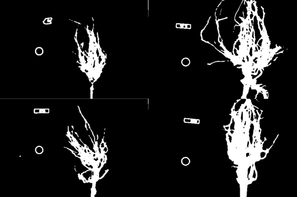
What is & doing in the solution above?

The & operator above means that we have defined a logical AND statement. This combines the two tests of pixel intensities in the blurred image such that both must be true for a pixel’s position to be set to True in the resulting mask.

Result of t < blurred_image	Result of blurred_image < 0.95	Resulting value in binary_mask
False	True	False
True	False	False
True	True	True

Knowing how to construct this kind of logical operation can be very helpful in image processing. The University of Minnesota Library’s guide to Boolean operators is a good place to start if you want to learn more.

Exercise: Thresholding a bacteria colony image (15 min)

In the images directory data/, you will find an image named colonies-01.tif.

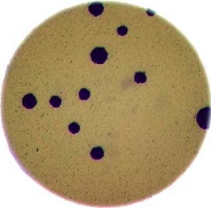
This is one of the images you will be working with in the morphometric challenge at the end of the workshop.

1. Plot and inspect the grayscale histogram of the image to determine a good threshold value for the image.

2. Create a binary mask that leaves the pixels in the bacteria colonies “on” while turning the rest of the pixels in the image “off”.

Solution

Here is the code to create the grayscale histogram:

bacteria = iio.imread(uri="data/colonies-01.tif")
gray_image = ski.color.rgb2gray(bacteria)
blurred_image = ski.filters.gaussian(gray_image, sigma=1.0)
histogram, bin_edges = np.histogram(blurred_image, bins=256, range=(0.0, 1.0))
fig, ax = plt.subplots()
ax.plot(bin_edges[0:-1], histogram)
ax.set_title("Graylevel histogram")
ax.set_xlabel("gray value")
ax.set_ylabel("pixel count")
ax.set_xlim(0, 1.0)

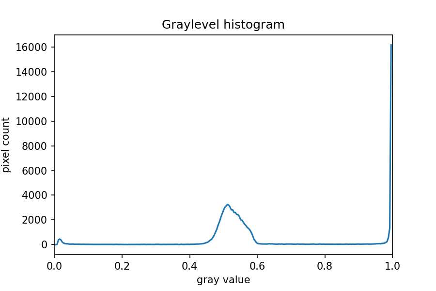
The peak near one corresponds to the white image background, and the broader peak around 0.5 corresponds to the yellow/brown culture medium in the dish. The small peak near zero is what we are after: the dark bacteria colonies. A reasonable choice thus might be to leave pixels below t=0.2 on.

Here is the code to create and show the binarized image using the < operator with a threshold t=0.2:

t = 0.2
binary_mask = blurred_image < t

fig, ax = plt.subplots()
ax.imshow(binary_mask, cmap="gray")

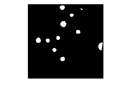
When you experiment with the threshold a bit, you can see that in particular the size of the bacteria colony near the edge of the dish in the top right is affected by the choice of the threshold.

Summary Quiz